It’s been over a year since we published the first global whole-genome snapshot of nearly 2000 genomes of the typhoid bacterium, Salmonella Typhi in Nature Genetics.
That paper focused on the emergence and global dissemination of what we’ve been calling for years the “H58” clone (see this blog post). This clone accounted for nearly half of all the isolates sequenced, and is a big deal because it tends to be multidrug resistant (MDR), carrying a suite of resistance genes that render all the cheap, first-line drugs like chloramphenicol, ampicillin, and trimethoprim-sufamethoxazole useless for treatment. Detailed genomic epi studies show the local impact of the arrival of MDR H58 in countries as widespread as Malawi and Cambodia; and the emergence of fluoroquinolone resistant H58 sublineage in India and Nepal recently stopped a treatment trial because the current standard of care – ciprofloxacin – was resulting in frequent treatment failure.
While H58 is important, the global Typhi population contains a lot of genomic diversity outside the H58 clone, and we’ve turned our attention to the rest of the population now in a new paper in Nature Communications: “An extended genotyping framework for Salmonella enterica serovar Typhi, the cause of human typhoid”
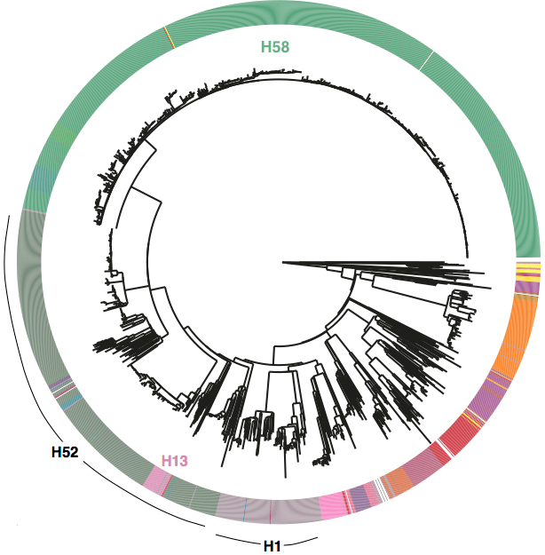
First, we decided that we needed to revisit the haplotyping scheme of Roumagnac et al (from which H58 gets its name), which was based on just ~80 genes, using the whole genome phylogeny. Here is the tree inferred from core genome SNPs in 1832 Typhi strains, with the old haplotypes indicated by the coloured ring around the outside. It’s pretty easy to see that some haplotypes (like H52 and H1) actually comprise multiple distinct phylogenetic lineages (low resolution), while others subdivide lineages (excessive resolution).

Whole genome SNP tree for 1832 strains, outer ring indicates haplotypes based on mutations in 80 genes as defined in Roumagnac et al, Science 2006.
We used BAPS to define genetic clusters at various levels (thanks to Tom Connor for running this). We settled on 3 levels of hierarchical clustering, indicated in the tree below:
• 4 nested primary clusters (inner-most ring; yellow, green, blue, red). These have 100% bootstrap support and are each characterised by >20 SNPs
• Clusters are further divided into 16 clades (middle ring and labels). The median pairwise distance between isolates in the same clade is 109 SNPs, while the inter-clade SNP distance averages 243 SNPs.
• Clades are further divided into 49 subclades, indicated by alternating background shading colours. The median pairwise distance between isolates in the same subclade is 25 SNPs.

Tree indicating new phylo-informed genotypes. Primary clusters 1-4 are indicated in the inner ring. Branch colours indicate clades, which are also labelled on the outside and coloured in the outer ring. Subclades are indicated by alternating background shading.
 One of the key reasons we wanted to define the phylogenetic lineages in this way is to make them easier to identify and talk about. I’ve always been a fan of MLST for this reason, since it’s much easier to talk about K. pneumoniae ST258, ST11, ST15 etc than ‘that lineage that has reference strain X in it’. So we introduce a hierarchical nomenclature system, similar to the one currently in use for Mycobacterium tuberculosis, where the 4 primary clusters (1, 2, 3, 4) are subdivided into 16 clades (1.1, 1.2; 2.1, 2.2, etc) which in turn are subdivided into 49 subclades (1.1.1, 1.1.2, etc). This has the advantage of conveying hierarchical relationships between groups – e.g. 2.2.1 and 2.2.2 are sister subclades within clade 2.2, which is a sister clade of 2.1.
The subclades are easier to distinguish in the collapsed rectangular tree on the right, where each subclade is represented by just one strain.
Some BAPS clusters were polyphyletic and consisted of isolates belonging to rare phylogenetic lineages whose common ancestor in the tree coincided with the common ancestor of an entire clade (n=9) or primary cluster (n=2). These groups contain isolates that, given increased numbers, may emerge as distinct clusters that form sister taxa within the parent clade (or primary cluster), and were given the suffix ‘.0’ rather than a defined cluster number (e.g. 3.0 or 3.1.0) to indicate non-equivalence with the properly differentiated sister clades (n=16) or subclades (n=49). As more genomes are added, these are expected to be more clearly differented into distinct groups and given proper clade/subclade designations.
Next we defined a set of 68 SNPs that can be used to genotype isolates into these groups. We chose one SNP for each primary cluster, clade and subclade (preferentially choosing intragenic SNPs in well-conserved core genes). The SNPs are detailed in a supplementary spreadsheet, and we provide a script to assign strains to genotypes based on an input BAM or VCF file generated by mapping to the reference genome for Typhi strain CT18.
An isolate that belongs to a differentiated subclade such as 2.1.4 will be hierarchically identified by carrying the derived allele for primary cluster 2 (but not the nested clusters 3 and 4); the derived allele for clade 2.1 (but no other clades) and the derived allele for subclade 2.1.4 (but no other subclades). It is possible for an isolate to carry derived alleles for a primary cluster and clade with no further differentiation into subclade.
The clone formally known as H58
Under the new scheme, the infamous H58 clone is named subclade 4.3.1, which so far has no sister clades. I suspect those of us familiar with Typhi population genomics will keep referring to it informally as H58 for some time, since that name is now well known… but I will try to re-train myself to call it 4.3.1 (H58).
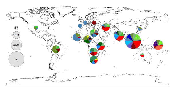
Now the fun part: exploring the geographical distribution of these lineages.

Figure 1c from the paper. Pie colours indicate clades found in each WHO region in the global data set (key is in the tree figure above).
In the paper we go on to show that:
• clades are widely geographically distributed, while subclades are geographically constrained (see heatmap below);
• genotyping can be used to predict the geographical origin of travel-associated typhoid in patients in London;
• even better predictions can be obtained based on genome-wide SNP distances to our reference panel of >1800 isolates… but of course that involves a lot more computationally intensive comparisons than a quick screen of a new isolate’s BAM file.

Figure 2 of the paper, showing the geographical distribution of subclades, which shows most subclades are restricted to a single region. For this analysis, the effect of local outbreaks has been minimised by replacing groups of strains that share the same subclade and year and country of isolation with a single representative strain.
You can read the full details in the paper, but here I just want to highlight that you can now explore the global genomic framework for Typhi – including genotype designations as well as temporal and geographic data – interactively in MicroReact.
How does genotyping help with studying local populations?
We have already begun using the new genotyping scheme in local typhoid studies. I find this a really helpful way to describe/summarise the local populations, and place them in the context of the global population without resorting to large trees.
For example in this recent Nigerian study, we described the population like this: “The majority of isolates (84/128, 66%) belonged to genotype 3.1.1 , which is relatively common across Africa, predominantly western and central countries. In the wider African collection genotype 3.1.1 was represented by isolates from neighbouring Cameroon and across West Africa (Benin, Togo, Ivory Coast, Burkina Faso, Mali, Guinea and Mauritania) suggesting long-term inter-country exchange within the region. Most of the remaining isolates belonged to four other genotypes (4.1, 2.2, 2.3.1 and 0.0.3).”
Of course genotype assignment is not the end of the story – we still want to build whole-genome trees to explore the relationships of local isolates with those from other countries. Importantly, working with genotypes means that we can achieve this without needing to build a megatree of all isolates in the local + global collections (n>2000). Instead, we can use the genotypes to identify which strains from the global collection are relatives of the Nigerian isolates, and build a much smaller tree that still captures all of the information about transmission/transfer between Nigeria and other countries:

The tree and map were made using MicroReact, you can recreate theme here: http://microreact.org/project/styphi_nigeria To get this colour scheme just click on the eye icon (bottom left) and select ‘country’; and to get the fan style tree, click the settings button (top right) and click the fan shape.
Another example is in our recent paper on isolates collected in Thailand before and after the introduction of their national vaccination program (pre-print here):
- Genotype 3.2.1 was the most common (n=14, 32%), followed by genotype 2.1.7 (n=10, 23%)
- Genotypes 2.0 (n=1, 2%) and 4.1 (n=3, 7%) were observed only in 1973 (pre-vaccine period)
- Genotypes 2.1.7 (n=10, 23%), 2.3.4 (n=1, 2%), 3.4.0 (n=2, 5%), 3.0.0 (n=3, 7%), 3.1.2 (n=2, 5%), were observed only after 1981 (post-vaccine period)
- Genotypes 3.2.1 and 2.4.0 were observed amongst both pre- and post-vaccine isolates, but the subclade phylogenies show that these more likely to represent re-introduction of strains from neighbouring countries than persistence within Thailand throughout the immunisation program.

