Gordon Dougan & Kat Holt
Making a COVID-19 vaccine will be a huge undertaking. We have outlined here, in some detail, the steps normally taken to make a vaccine and compare this to what may happen for COVID-19.

I’m currently on holiday in Japan after attending the excellent 2nd SMBE Satellite Workshop on Genome Evolution in Pathogen Transmission and Disease in Kyoto.
Before all the memories fade away with the magic of Japanese onsen, sake, ramen etc I wanted to record some of the highlights.
For me the greatest thing was seeing several invited speakers sharing their talk slots, tag-team style, with members of their lab. Perhaps this wouldn’t work in a more formal conference setting but in this workshop style event it was truly fantastic, and I hope to see more of it (and I look forward to doing it myself too – I didn’t on this occasion because I wasn’t presenting).
Here are some other highlights are in no particular order…
Let’s hope we get to come back to Japan for a third workshop soon…
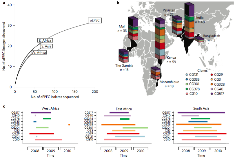
Today I’m pleased to see the final version of our paper on antimicrobial resistance in intestinal E. coli from Asian & African children published in Nature Microbiology. This is last piece of the puzzle from Danielle Ingle’s PhD research, a tremendous effort centred around the analysis of a collection of ~200 atypical enteropathogenic E. coli (aEPEC) isolated from cases and controls in seven countries during the Global Enterics Multicentre Study (GEMS).
The first analysis of the genome data from this collection was reported in this 2016 paper, also in Nature Microbiology. It focused on understanding the population structure of the pathotype, including establishing a framework for looking at variation in the primary virulence locus (the LEE pathogenicity island; see blog post here).
Danielle then looked at serotype diversity in the collection, and used the experience to tackle the problem of O and H serotype prediction from genome data. That work is detailed in this Microbial Genomics paper, which utilises the phenotypes and genome data from the GEMS aEPEC collection to assess the reliability of predictions.
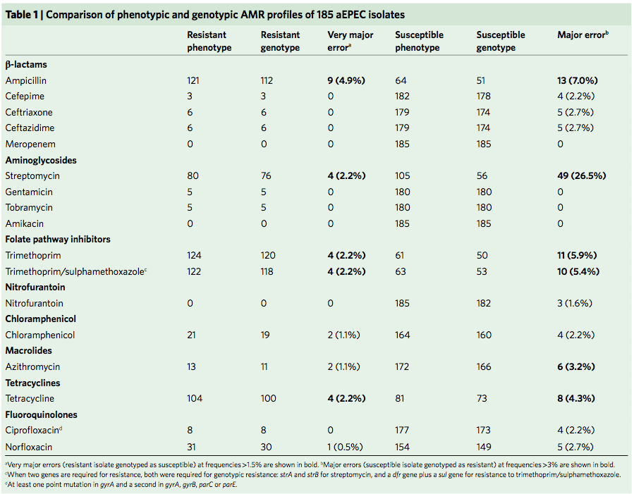
Finally we turned our attention to antimicrobial resistance (AMR) in the isolate collection – characterising resistance phenotypes, looking at known genetic determinants of AMR in the genome data, and also examining data on prescribing of antimicrobials for treatment of diarrhoeal disease in children at each study site.
So what did we find?
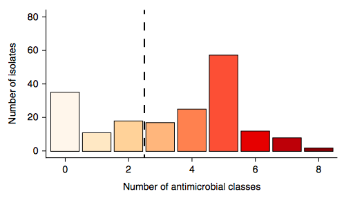
Firstly, whether we consider AMR phenotypes or genotypes we see that AMR was rampant, with most strains either multidrug resistant (65%; resistan to ≥ 3 drug classes) or susceptible to all drugs tested (19%):
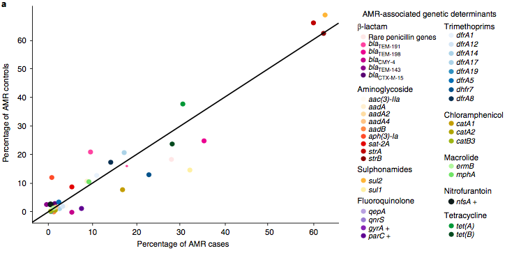
We found >40 different acquired AMR genes in the genomes, and also point mutations that are known to be associated with resistance to fluoroquinolones (in gyrA, parC) or nitrofurantoin (nfsA). Notably there was no difference between AMR rates in cases and controls, even at the level of individual genes:
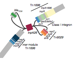
We found that many of these AMR genes co-occured together in known mobile genetic elements:
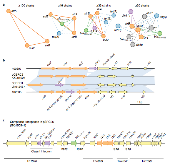
Quite often the structures of these elements were not totally resolvable from the genome assemblies, which were based on short Illumina reads only (no long reads for this data set unfortunately!)… but nevertheless, Danielle could often resolve co-localisation of these genes from the assembly graphs using Bandage:
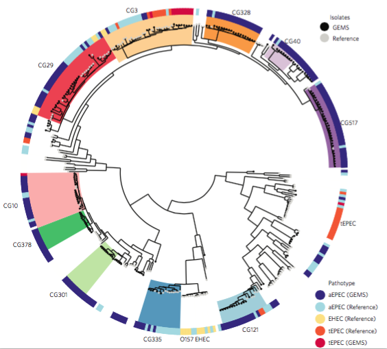
We had seen in the first paper that the isolates were highly diverse, comprising dozens of distinct clones… this tree is inferred from a core gene alignment of the study isolates together with some other genomes for context (GEMS study isolates are indicated as dark blue in the outer ring). The ten shaded clades indicate dominant clonal groups in the study population.
Back to the AMR study. We did a discriminant analysis of principle components (DAPC) to see whether the variation in the distribution of genetic determinants amongst the genomes could be used to discriminate between the clonal groups, and saw that AMR was not associated with individual clones:
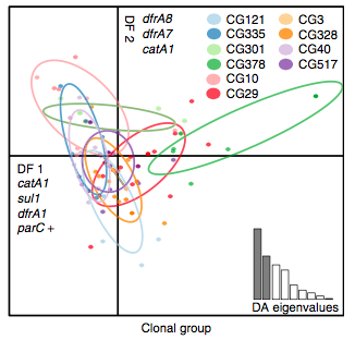
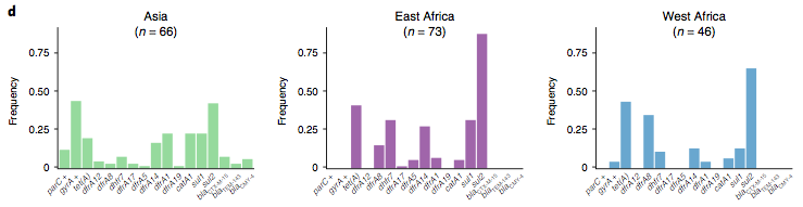
Instead we found that variation in AMR gene complement could discriminate isolates from different geographical region, suggesting that AMR genes more often reflect horizontal acquisition from distinct local gene pools in different parts of the world, rather than fixed features of their host bacterium that travel the world with their host strain (clone):
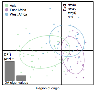
In particular, we saw that fluoroquinolone resistance associated mutations in gyrA were associated with Asian sites; while sites in East vs West Africa could be discriminated by the presence of different dihydrofolate reductase (dfr) genes responsible for trimethoprim resistance, with dfrA8 being more common in West Africa and dfrA5 being present in East Africa.
The data we have showed regional differences in AMR phenotypes, and in antibiotic usage for treatment of paediatric diarrhoea at the GEMS sites.
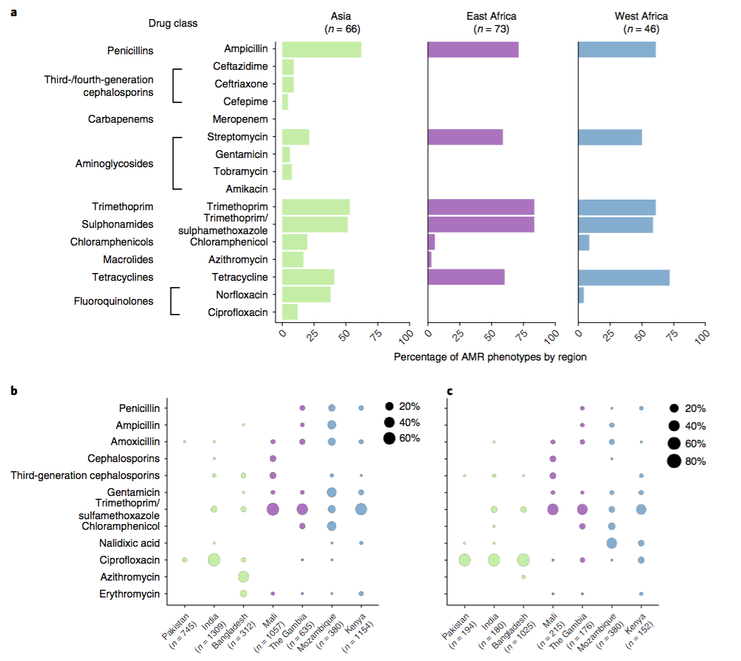
a) Resistance phenotypes. b) Frequency of antimicrobials prescribed to children with watery diarrhoea. c) Frequency of antimicrobials prescribed to children with dysentery.
However the prevalence of acquired resistance genes amongst E. coli isolated from each site was not associated with local frequencies of drug usage. The exception was fluoroquinolones: point mutations in gyrA and parC (which reduce MIC to ciprofloxacin) were more common at the Asian sites, where ciprofloxacin was used much more often to treat diarrheal disease than in African sites.
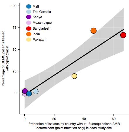
There are many possible reasons for the lack of association between local prescribing for diarrheal disease and the presence of AMR genes in local diarrheal pathogens. We expect that most antimicrobial exposure in human gut bugs like E. coli probably is not associated with attempts to treat E. coli infection at all, but with exposure to drugs given to treat other infections, drugs used in food animals which are a reservoir for E. coli, or even environmental contamination with antibiotics. Also because the horizontally acquired genes tend to travel together as a group in mobile genetic elements, exposure to one drug can co-select for resistance to many. This may be one reason that the association was more evident for ciprofloxacin use and gyrA/parC mutations, which are not in linkage with acquired AMR genes.
Finally, the data provided an opportunity to explore how well we can predict AMR phenotypes based on identifying known genetic determinants of AMR in E. coli genomes. The results were pretty good, indicating low rates of “very major errors” (where we predict a strain to be susceptible, but really it is resistant) for most drug classes. These results are comparable to those done independently in other collections of E. coli and also other bacteria, summarised here. But clearly there is room for improvement, and probably a few new mechanisms floating around out there… notably we didn’t aim to assess changes in expression of intrinsic E. coli genes, such as efflux pumps and beta-lactamases, which can contribute to drug resistance but are not so easy to find in genome data.
by David Edwards
In 2013, Kat and I wrote what turned out to be a very popular Beginner’s guide for comparative bacterial genome analysis. After four years and 120,000+ downloads of the guide, we thought it might be time to update the hands-on tutorial that was included.
As with any science, there have been advances in this time. We don’t have time to update all aspects, but felt it was important to update the recommended assembler from Velvet to SPAdes. The latter has become the ‘go-to’ assembler with our lab and many others over the last few years. Unfortunately, SPAdes does not work with Windows, but Windows users can use the original Velvet assembler if they wish to attempt their own assembly.
Also, Ryan Wick in our lab has developed a way to visualise the assembly graphs produced by SPAdes and other assemblers, in the form of a software program called Bandage. This allows us to examine and compare the properties of assembly graphs, useful if you are trying to assemble the same set of reads with different methods or parameter settings.
The other changes in version 2 are mainly to fix broken links to the E. coli sequences that have now been archived by NCBI, kindly pointed out to us by Michael Hall and others via email.
We continue to recommend Artemis and ACT for visualising and comparing annotated bacterial genome sequences, and both tools are still actively maintained at the Sanger Institute. While BRIG is no longer actively maintained, we continue to recommend it as it appears to be stable across newer versions of Java and BLAST, and it remains incredibly useful.
Hands-on tutorial v2 (6 Mb PDF): ComparativeGenomicsTutorialV2
Original article: Beginner’s guide to comparative bacterial genome analysis using next-generation sequence data
It’s been over a year since we published the first global whole-genome snapshot of nearly 2000 genomes of the typhoid bacterium, Salmonella Typhi in Nature Genetics.
That paper focused on the emergence and global dissemination of what we’ve been calling for years the “H58” clone (see this blog post). This clone accounted for nearly half of all the isolates sequenced, and is a big deal because it tends to be multidrug resistant (MDR), carrying a suite of resistance genes that render all the cheap, first-line drugs like chloramphenicol, ampicillin, and trimethoprim-sufamethoxazole useless for treatment. Detailed genomic epi studies show the local impact of the arrival of MDR H58 in countries as widespread as Malawi and Cambodia; and the emergence of fluoroquinolone resistant H58 sublineage in India and Nepal recently stopped a treatment trial because the current standard of care – ciprofloxacin – was resulting in frequent treatment failure.
While H58 is important, the global Typhi population contains a lot of genomic diversity outside the H58 clone, and we’ve turned our attention to the rest of the population now in a new paper in Nature Communications: “An extended genotyping framework for Salmonella enterica serovar Typhi, the cause of human typhoid”
First, we decided that we needed to revisit the haplotyping scheme of Roumagnac et al (from which H58 gets its name), which was based on just ~80 genes, using the whole genome phylogeny. Here is the tree inferred from core genome SNPs in 1832 Typhi strains, with the old haplotypes indicated by the coloured ring around the outside. It’s pretty easy to see that some haplotypes (like H52 and H1) actually comprise multiple distinct phylogenetic lineages (low resolution), while others subdivide lineages (excessive resolution).
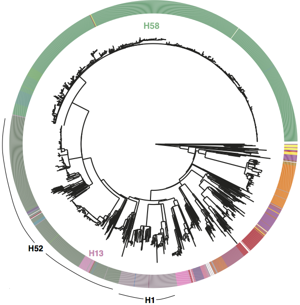
Whole genome SNP tree for 1832 strains, outer ring indicates haplotypes based on mutations in 80 genes as defined in Roumagnac et al, Science 2006.
We used BAPS to define genetic clusters at various levels (thanks to Tom Connor for running this). We settled on 3 levels of hierarchical clustering, indicated in the tree below:
• 4 nested primary clusters (inner-most ring; yellow, green, blue, red). These have 100% bootstrap support and are each characterised by >20 SNPs
• Clusters are further divided into 16 clades (middle ring and labels). The median pairwise distance between isolates in the same clade is 109 SNPs, while the inter-clade SNP distance averages 243 SNPs.
• Clades are further divided into 49 subclades, indicated by alternating background shading colours. The median pairwise distance between isolates in the same subclade is 25 SNPs.
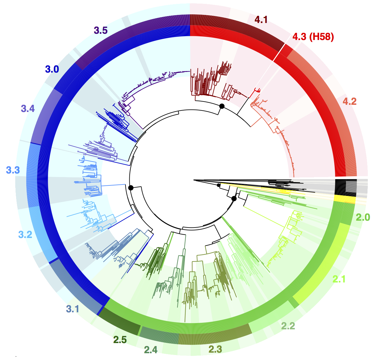
Tree indicating new phylo-informed genotypes. Primary clusters 1-4 are indicated in the inner ring. Branch colours indicate clades, which are also labelled on the outside and coloured in the outer ring. Subclades are indicated by alternating background shading.
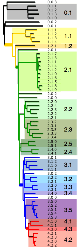 One of the key reasons we wanted to define the phylogenetic lineages in this way is to make them easier to identify and talk about. I’ve always been a fan of MLST for this reason, since it’s much easier to talk about K. pneumoniae ST258, ST11, ST15 etc than ‘that lineage that has reference strain X in it’. So we introduce a hierarchical nomenclature system, similar to the one currently in use for Mycobacterium tuberculosis, where the 4 primary clusters (1, 2, 3, 4) are subdivided into 16 clades (1.1, 1.2; 2.1, 2.2, etc) which in turn are subdivided into 49 subclades (1.1.1, 1.1.2, etc). This has the advantage of conveying hierarchical relationships between groups – e.g. 2.2.1 and 2.2.2 are sister subclades within clade 2.2, which is a sister clade of 2.1.
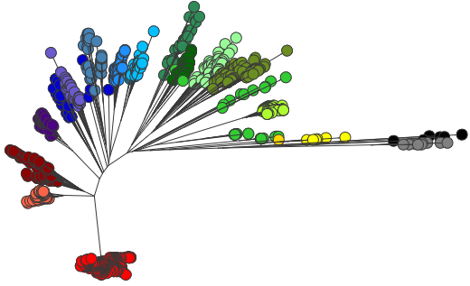
The subclades are easier to distinguish in the collapsed rectangular tree on the right, where each subclade is represented by just one strain.
Some BAPS clusters were polyphyletic and consisted of isolates belonging to rare phylogenetic lineages whose common ancestor in the tree coincided with the common ancestor of an entire clade (n=9) or primary cluster (n=2). These groups contain isolates that, given increased numbers, may emerge as distinct clusters that form sister taxa within the parent clade (or primary cluster), and were given the suffix ‘.0’ rather than a defined cluster number (e.g. 3.0 or 3.1.0) to indicate non-equivalence with the properly differentiated sister clades (n=16) or subclades (n=49). As more genomes are added, these are expected to be more clearly differented into distinct groups and given proper clade/subclade designations.
Next we defined a set of 68 SNPs that can be used to genotype isolates into these groups. We chose one SNP for each primary cluster, clade and subclade (preferentially choosing intragenic SNPs in well-conserved core genes). The SNPs are detailed in a supplementary spreadsheet, and we provide a script to assign strains to genotypes based on an input BAM or VCF file generated by mapping to the reference genome for Typhi strain CT18.
An isolate that belongs to a differentiated subclade such as 2.1.4 will be hierarchically identified by carrying the derived allele for primary cluster 2 (but not the nested clusters 3 and 4); the derived allele for clade 2.1 (but no other clades) and the derived allele for subclade 2.1.4 (but no other subclades). It is possible for an isolate to carry derived alleles for a primary cluster and clade with no further differentiation into subclade.
The clone formally known as H58
Under the new scheme, the infamous H58 clone is named subclade 4.3.1, which so far has no sister clades. I suspect those of us familiar with Typhi population genomics will keep referring to it informally as H58 for some time, since that name is now well known… but I will try to re-train myself to call it 4.3.1 (H58).
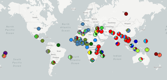
Now the fun part: exploring the geographical distribution of these lineages.
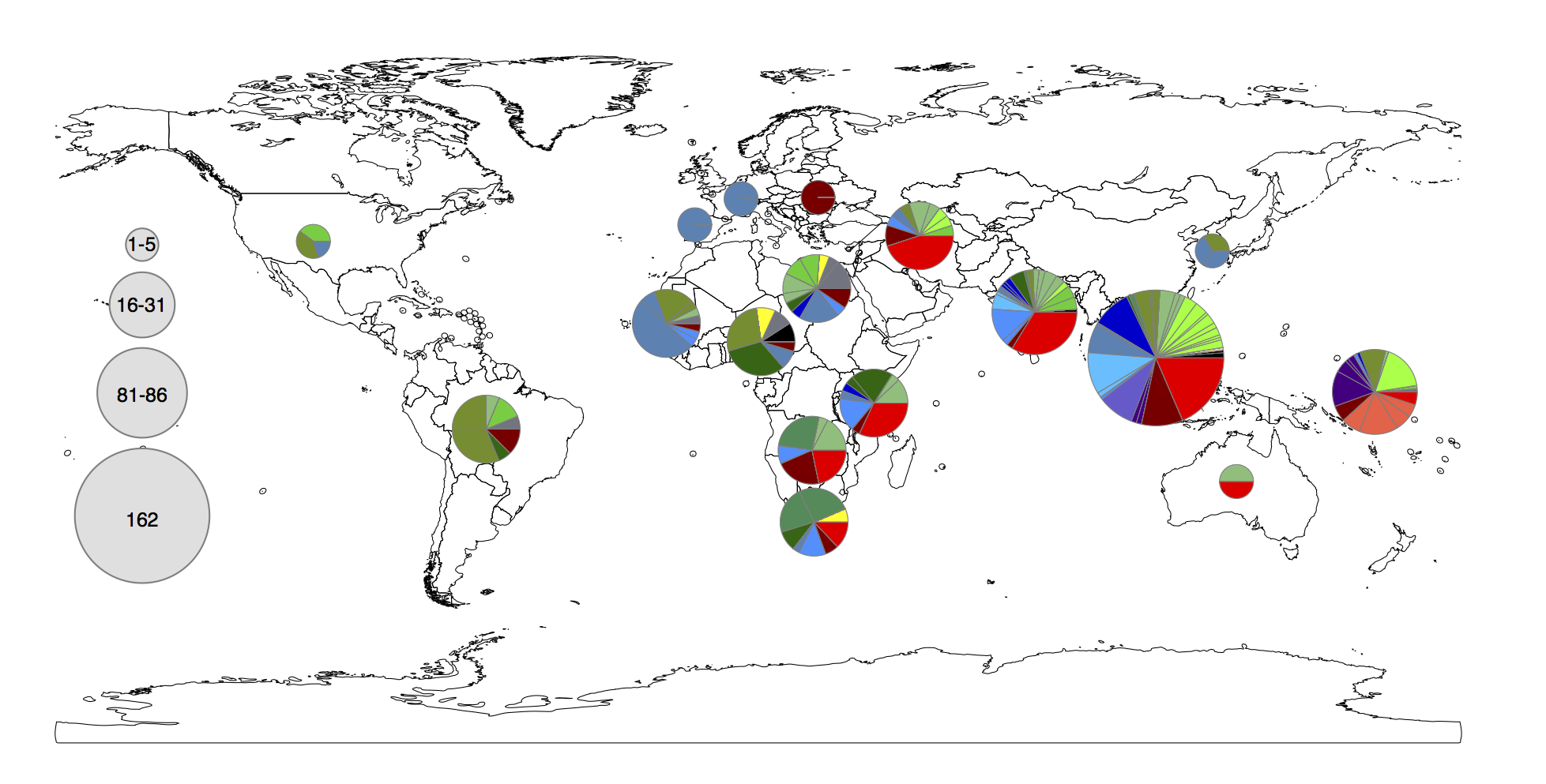
Figure 1c from the paper. Pie colours indicate clades found in each WHO region in the global data set (key is in the tree figure above).
In the paper we go on to show that:
• clades are widely geographically distributed, while subclades are geographically constrained (see heatmap below);
• genotyping can be used to predict the geographical origin of travel-associated typhoid in patients in London;
• even better predictions can be obtained based on genome-wide SNP distances to our reference panel of >1800 isolates… but of course that involves a lot more computationally intensive comparisons than a quick screen of a new isolate’s BAM file.
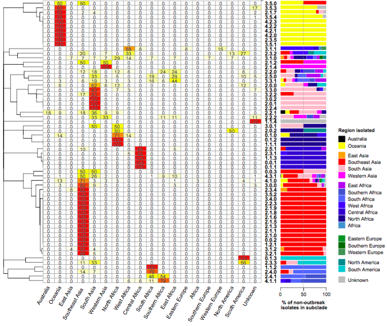
Figure 2 of the paper, showing the geographical distribution of subclades, which shows most subclades are restricted to a single region. For this analysis, the effect of local outbreaks has been minimised by replacing groups of strains that share the same subclade and year and country of isolation with a single representative strain.
You can read the full details in the paper, but here I just want to highlight that you can now explore the global genomic framework for Typhi – including genotype designations as well as temporal and geographic data – interactively in MicroReact.
How does genotyping help with studying local populations?
We have already begun using the new genotyping scheme in local typhoid studies. I find this a really helpful way to describe/summarise the local populations, and place them in the context of the global population without resorting to large trees.
For example in this recent Nigerian study, we described the population like this: “The majority of isolates (84/128, 66%) belonged to genotype 3.1.1 , which is relatively common across Africa, predominantly western and central countries. In the wider African collection genotype 3.1.1 was represented by isolates from neighbouring Cameroon and across West Africa (Benin, Togo, Ivory Coast, Burkina Faso, Mali, Guinea and Mauritania) suggesting long-term inter-country exchange within the region. Most of the remaining isolates belonged to four other genotypes (4.1, 2.2, 2.3.1 and 0.0.3).”
Of course genotype assignment is not the end of the story – we still want to build whole-genome trees to explore the relationships of local isolates with those from other countries. Importantly, working with genotypes means that we can achieve this without needing to build a megatree of all isolates in the local + global collections (n>2000). Instead, we can use the genotypes to identify which strains from the global collection are relatives of the Nigerian isolates, and build a much smaller tree that still captures all of the information about transmission/transfer between Nigeria and other countries:

The tree and map were made using MicroReact, you can recreate theme here: http://microreact.org/project/styphi_nigeria To get this colour scheme just click on the eye icon (bottom left) and select ‘country’; and to get the fan style tree, click the settings button (top right) and click the fan shape.
Another example is in our recent paper on isolates collected in Thailand before and after the introduction of their national vaccination program (pre-print here):