Author: kat

Bacterial genomics researcher in Melbourne, Australia

Elizabethkingia anophelis

DATA: raw Illumina reads (CDC) under SRP072035

Assemblies & analyses: https://github.com/katholt/elizabethkingia

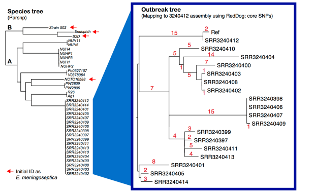
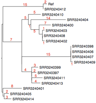
Left – core SNP tree, created from assembled genomes using Parsnp. Right – core SNP tree, created by mapping all outbreak genomes to our 9-contig assembly for SRR3240412, using our RedDog pipeline. Details below; all assemblies and mapping outputs are here.

March 19, 2016: I saw on twitter today that there was an outbreak of a weird bacteria I’ve never heard of before (Elizabethkingia anophelis) in Wisconsin, which had infected >50 people and killed almost 20.

The Wisconsin Health Services department has posted some information here (click the “For Health Professionals” tab to get info on the bacteria and antibiotic resistance).

CDC has deposited Illumina reads from 18 outbreak strains into SRA under project SRP072035 so I pulled the data and had a look. I managed to download the readsets in a few minutes (using bionode-ncbi) but it took a really long time to unpack these into fastq files using sra-toolkit.

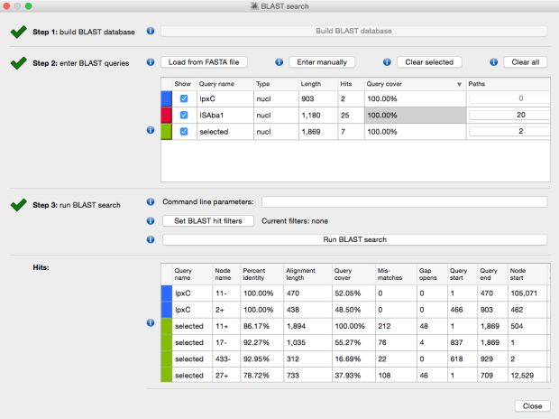
As I have no idea about this species, I thought I’d start by looking for antibiotic resistance and plasmids in the first 6 read sets using our SRST2 software, while waiting for the rest of the reads to unpack… this ran quickly and showed me the same results for all 6 strains: GOB-10 (1 SNP from the closest allele in the ARG database) and B-2 (3 SNPs), at depths of 35-65x. For example:

SRR3240397 ARGannot.r1 GOB-1_Bla GOB-10_821 100.0 47.59 1snp 0.115 873 0.043 188 821 no;yes;GOB-10;Bla;AY647247;1-873;873
SRR3240397 ARGannot.r1 B-1_Bla B-2_1160 100.0 59.891 3snp 0.4 750 0.03 314 1160 no;no;B-2;Bla;AF189300;1-750;750

Because the matches were not identical, I pulled the consensus sequences (based on read mapping) using –report_all_consensus option in SRST2:

>314__B-1_Bla__B-2__1160 no;no;B-2;Bla;AF189300;1-750;750
ATGTTGAAAAAAATAAAAATAAGCTTGATTCTTGCTCTTGGGCTTACCAGTCTGCAGGCA
TTTGGACAGGAGAATCCTGACGTTAAAATTGATAAGCTAAAAGATAATCTGTATGTATAC
ACAACCTACAATACATTTAACGGGACTAAATATGCCGCTAATGCAGTATATCTGGTAACT
GATAAGGGTGTTGTGGTTATAGACTGTCCGTGGGGAGAAGACAAATTTAAAAGCTTTACG
GACGAGATTTATAAAAAACACGGAAAGAAAGTTATTATGAATATTGCAACACATTCTCAT
GATGATCGTGCCGGAGGTCTTGAATATTTTGGTAAAATAGGTGCAAAAACTTATTCTACT
AAAATGACAGATTCTATTTTAGCAAAAGAGAATAAGCCAAGAGCACAATATACTTTTGAC
AATAATAAATCTTTCAAAGTAGGAAAATCCGAGTTTCAGGTTTACTATCCCGGAAAAGGA
CATACAGCAGATAATGTGGTGGTATGGTTTCCAAAAGAAAAAGTATTGGTTGGAGGTTGT
ATTATAAAAAGCGCTGATTCAAAAGACCTGGGGTATATTGGAGAAGCATATGTAAACGAC
TGGACGCAGTCTGTACACAATATTCAACAAAAGTTTTCCGGTGCTCAGTACGTTGTTGCA
GGGCATGATGATTGGAAAGATCAAAGATCAATACAACGTACACTAGACTTAATCAATGAA
TATCAACAAAAACAAAAGGCTTCAAATTAA

>188__GOB-1_Bla__GOB-10__821 no;yes;GOB-10;Bla;AY647247;1-873;873
ATGAGAAATTTTGTTATACTGTTTTTCATGTTCATTTGCTTGGGCTTGAATGCTCAGGTA
GTAAAAGAACCTGAAAATATGCCCAAAGAATGGAACCAGACTTATGAACCCTTCAGAATT
GCAGGTAATTTATATTACGTAGGAACCTATGATTTGGCTTCTTACCTTATTGTGACAGAC
AAAGGCAATATTCTCATTAATACAGGAACGGCAGAATCGCTTCCAATAATAAAAGCAAAT
ATCCAAAAGCTCGGGTTTAATTATAAAGACATTAAGATCTTGCTGCTTACTCAGGCTCAC
TACGACCATACAGGTGCATTACAAGATCTTAAAACAGAAACCGGTGCAAAATTCTATGCC
GATAAAGAAGATGCTGATGTCCTGAGAACAGGGGGGAAGTCCGATTATGAAATGGGAAAA
TATGGGGTGACATTTAAACCTGTTACTCCGGATAAAACATTGAAAGATCAGGATAAAATA
ACACTGGGAAATACAATCCTGACTTTGCTTCATCATCCCGGACATACAAAAGGTTCCTGT
AGTTTTATTTTTGAAACAAAAGACGAGAAGAGAAAATATAGAGTTTTGATAGCTAATATG
CCCTCCGTTATTGTTGATAAGAAATTTTCTGAAGTTACCGCATATCCAAATATTCAGTCC
GATTATGCATATACTTTCAAAGCAATGAAGAATCTGGATTTTGATATTTGGGTGGCCTCC
CATGCAAGTCAGTTCGATCTCCATGAAAAACGTAAAGAAGGAGATCCGTACAATCCGCAA
TTGTTTATGGATAAGCAAAGCTATTTCCAAAACCTTAATGATTTGGAAAAAAGCTATCTC
GACAAAATAAAAAAAGATTCCCAAGATAAATAA

I had a quick look at the accessions for these genes (they are hiding in the fasta headers above) and found that they are carbapenemase genes reported from Elizabethkingia meningosepticum (previously called Chryseobacterium meningosepticum), reported in these papers: Bellais 2000, Antimicrob. Agents Chemother and Yum 2010, J Microbiol. These genes confer resistance to carbapenems like meropenem and imipenem, which probably contributes to these bacteria causing hospital-acquired infections as they will be selected for by carbapenem exposure.

SRST2 didn’t find any other acquired antibiotic resistance genes (from the ARG-Annot database) or known plasmid replicons (at least those in the PlasmidFinder database), which is consistent with the Wisconsin health services reports that these strains are susceptible to lots of readily accessible drugs including fluoroquinolones, rifampin and trimethoprim/sulfamethoxazole.

Running a quick NCBI BLAST search of the carbapenemase gene sequences shows that these new sequences, which are from outbreak strains identified definitively as Elizabethkingia anophelis by CDC, are closest to sequences annotated in NCBI as originating from Elizabethkingia meningosepticum. (The trees below are just straight out NCBI BLAST, obtained by clicking “Distance tree of results” and then downloading the newick tree files to view in FigTree.)

Screen Shot 2016-03-19 at 4.21.25 pm

The outbreak strain’s GOB-10 gene had 1 synonymous SNP compared to the reference sequence, while the B-2 gene had 1 synonymous and 2 non-synonymous SNPs (affecting codons 31 & 34, which is outside the beta-lactamase domain).

I am guessing that species assignations are pretty tricky for this genus, as few labs will have access to definitive tests to discern them, so we shouldn’t read much into this. However if it is true that the outbreak strains are Elizabethkingia anophelis and the close-matching genes in NCBI did come from Elizabethkingia meningosepticum, this would suggest that there is horizontal gene transfer between these species.

Note 1: while writing this, the fastqs finished extracting and I ran SRST2 and found the same antibiotic resistance gene results on all 18. I’m now running some SPAdes assemblies which I’ll post here later, to save others the trouble…

Note 2: the assemblies (SPAdes fasta and fastg; plus Prokka annotated in GenBank format), and various analyses including trees created using Parsnp (from assemblies) and our RedDog pipeline (mapping of reads to reference genome strain NUHP1 =CP007547) are here in github: https://github.com/katholt/elizabethkingia

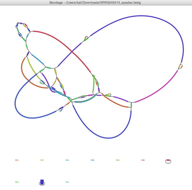
The assemblies are a bit variable, but mostly ~3.9 Mbp (the reference is 4,369,828) but the best one was for SRR3240413 – 32 contigs with 3,911,053 bp total. Viewing the SPAdes assembly graph in our Bandage program shows that 3,910,660 bp are in a single linked graph, which corresponds to the chromosome. (The other little bits do not look like plasmids, just leftover bits of sequence and probably adapters, that SPAdes spit out in teeny bits of a few hundred bp each.)

SRR3240413_bandage_graph

The genomes look pretty similar at first glance, but interestingly 4 of them share a deletion of ~80 genes. That’s a great little epidemiological marker for the investigations.

Screen Shot 2016-03-19 at 7.24.21 pm

This was detected by our mapping pipeline RedDog, which I used to map the reads to reference genome NUHP1 CP007547 (this may not be the best reference, I just picked one randomly). The assemblies confirm it: genes BD94_0888 to BD94_0962, and the end of BD94_0963, are missing in these 4 strains (although reads do map to BD94_0948, because this is present in a second copy elsewhere in the genome).

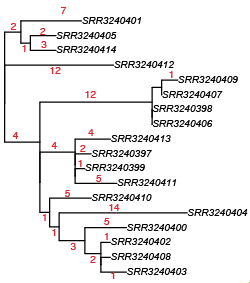
Here’s that tree with a bit more detail (red = # core SNPs). The tree was made using FastTree, with NUHP1 reference genome as an outgroup (the outbreak strains are >40,000 SNPs away from this reference).

Screen Shot 2016-03-19 at 8.26.50 pm

UPDATE 20/3

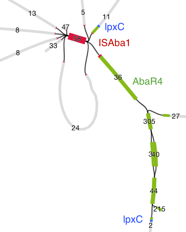
David Edwards has been playing with Hybrid StriDe + SPAdes assembly recently, and tried this with SRR3240412. The SPAdes assembly (here) was 3,913,666 bp in 41 contigs. The hybrid assembly (here) is 3,917,367 bp in 9 contigs. This is what the graph looks like… I’m showing it coloured by BLAST matches to the NUPH1 reference genome so you can see what the likely path through the graph is (rainbow, red -> purple, indicates matches from start -> end coordinates of the reference genome).

March 22: Hybrid assemblies for all 18 outbreak genomes (9-15 contigs each; ranging 3,830,044 – 3,912,928 bp) are now in GitHub (thanks to David Edwards for this).

David re-ran the RedDog mapping pipeline using this genome assembly as the reference, and got a very similar tree (files in GitHub):

SRR3240412_RedDogTree

And here is a core genome SNP tree (made from genome assemblies using Harvest), which shows the outbreak strains are a novel lineage of E. anophelis, compared to currently available data (tree file in GitHub):

species_tree_with_NCTC10588

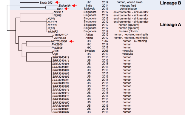
Note: Sylvain Brisse has shown the same thing using his core genome MLST scheme (see BioRxiv preprint posted March 19). I have used his nomenclature here (lineage A, lineage B). Note that Lineage B strains were originally identified as E. meningoseptica, but belong to E. anophelis. I have also included here the genome of E.meningoseptica NCTC10588, which was sequenced as part of the Sanger/PHE/PacBio type strain project, in this tree… it clusters within lineage A and is clearly E. anophelis.

UPDATE: This tweet-fest led to a collaborative project between myself, Sylvain Brisse (Institut Pasteur) and CDC, which was eventually published in Nature Communications a year after this blog post: “Evolutionary dynamics and genomic features of the Elizabethkingia anophelis 2015 to 2016 Wisconsin outbreak strain”

Genomics of atypical enteropathogenic E. coli

Well our paper on “atypical” enteropathogenic E. coli is finally out, in the new journal Nature Microbiology. The hard work on this paper was done by Danielle Ingle, whom I co-supervise together with Roy Robins-Browne and will soon become the first of my students to complete a PhD. Unfortunately the paper is paywalled at the moment, so I’ll try to summarise the key elements here.

For those who aren’t familiar with the wacky world of E. coli pathotypes, the LEE genomic island is the darling of E. coli pathogenicity genetics. It encodes a type three secretion system, essentially a syringe structure that enables the bacteria to inject its own proteins (known as secreted effector proteins) directly into human cells and – ahem – mess them up (for more technical details see the impressive body of work from Melbourne University’s very own Jacqueline Pearson and Liz Hartland). E. coli that possess shiga toxin as well as the LEE cause nasty bloody diarrhoea and are defined as enterohaemorrhagic E. coli (EHEC), while those with LEE + the bfp adhesion factor cause diarrhoea and are defined as enteropathogenic E. coli (EPEC). Strains carrying the LEE but lacking both shiga toxin and bfp can also cause diarrhoea, but are also sometimes isolated from healthy individuals with no symptoms of diarrhoaea, and it is this big group of LEE + ??? strains that are defined as atypical EPEC (aEPEC), while those with bfp are dubbed typical EPEC.

No one has been able to find a common virulence factor that differentiates diarrhoeagenic aEPEC from asymptomatic strains… which is not that surprising considering that aEPEC is really just an umbrella term for a diverse group of organisms that happen to carry the LEE genomic island.

In this paper, we set out to define the population structure of aEPEC strains using genomics, and also to investigate variation in the LEE island itself. Our strain set is ~200 newly sequenced aEPEC that were isolated from children with diarrhoea, and from asymptomatic age-matched controls, as part of the Global Enteric Multicenter Study (GEMS) – a massive study into the etiology of childhood diarrhoea across seven sites in Africa and Asia, funded by the Gates Foundation. We also included lots of publicly available genomes from NCBI, which included ~60 additional aEPEC.

So what did we find? Well from a population structure point of view, we confirmed what we suspected from the beginning – that the ~200 aEPEC strains actually represent dozens of distinct lineages or clonal groups within the E. coli whole genome phylogeny. We tried making the core genome tree in a few different ways, including mapping reads to a reference genome vs using Roary to generate core gene alignments from assemblies; with and without removing recombinant regions identified using ClonalFrameML. The alternative trees all tell the same population structure story, as you can see below. An interactive version of the mapping-based, recombination-filtered tree (which appears in Figure 1 of the paper, panel a below) is available to play with in MicroReact.

Supplementary Figure 1

The 10 clades highlighted in the tree are those containing >5 aEPEC in our collection, which represent the most common aEPEC lineages. The figures below show that these 10 aEPEC groups are present across the Asian and African GEMS sites; most also appear in non-GEMS collections from Europe as well as North and South America, indicating they are globally distributed.

aEPEC_distribution

Next we looked in depth at the LEE genomic island itself. ClonalFrame analysis identified lots of recombination across the locus, particularly affecting the proteins that make direct contact with host cells:

Screen Shot 2016-01-19 at 9.46.45 am

Danielle also did a lot of work to examine selection pressures on the various LEE genes, and found evidence for co-evolutionary constraints on groups of LEE genes (see the paper for details).

We used the recombination-free ClonalFrame tree, which represents the underlying clonal or vertical evolutionary relationships between LEE sequences, to define LEE lineages and subtypes. We also made a MLST-style scheme for the LEE, to make it easy to identify types from sequence data without having to compare to reference trees. The sequence files are included in the SRST2 distribution and can be downloaded from https://github.com/katholt/srst2.

Screen Shot 2016-01-19 at 9.50.41 am

There were three clearly distinct LEE lineages, separated from one other by 4-7% divergence (similar to genus-level differences between bacteria) and with different preferences for chromosomal insertion site. One of the LEE lineages (lineage 1) was entirely novel and we found it only in aEPEC isolates from the GEMS study. Functionality of the LEE was confirmed in all GEMS strains, including these novel lineage 1 examples.

Importantly, different aEPEC lineages had distinct LEE variants, often integrated at different chromosomal sites, confirming that aEPEC lineages have evolved numerous times independently via distinct LEE acquisition events. Also, some aEPEC lineages contained strains carrying different LEE lineages and/or subtypes, sometimes integrated at different sites, indicating ongoing evolution within some aEPEC clades.

aEPEC_tree_LEE_subtypes

Unsurprisingly, some of the “aEPEC” lineages also include examples of EHEC and/or typical EPEC isolates, i.e. subclades within the LEE-containing lineage that have subsequently acquired shiga toxin (via phage) or a bfp plasmid. We also found extensive variation in the complement of known LEE-secreted effectors (which are scattered around the genome and known as non-LEE encoded effectors or nle genes), both within and between lineages.

There’s lots more work to do to unravel the genetic basis for pathogenicity in E. coli, including identifying more of the colonisation factors, regulators and effectors that are important for causing disease in humans. But I think this analysis is a great step towards clarifying the population structure of EPEC and the LEE more generally, which opens the door for much more informative diagnostics and epidemiological studies. This work should also help immensely in guiding future pathogenicity research… most research on EPEC or EHEC pathogenicity has so far focused on a handful of strains, but our genomic analysis shows there is a much wider diversity of strain backgrounds, LEE variants and effector gene content that also needs to be considered.

Microbial Genomics methods

MGen (Microbial Genomics) was created last year by the UK’s Microbiology Society, with the aim of becoming the go-to journal for microbial genomics research. As a Senior Editor, I was asked to help mark the occasion of MGen’s six month anniversary (on Jan 15, 2016), by reviewing the 24 papers published in the journal’s first six months since launch.
The full review is is available over on the MGen site, but I wanted to draw particular attention here to trends in the analysis tools used by the genomic epidemiology papers published so far in MGen, which largely reflects what’s been happening across the field generally.

tools word cloud

One third of the articles are cutting edge genomic epidemiologyin action, using genomics to investigate the evolution and transmission of a range of pathogens, from anthrax to dysentery and food poisoning.

Interestingly all of these studies used similar methodologies, reflecting the maturity of this field of research.

Common approaches include: (i) sequencing large numbers of isolates using high-throughput Illumina platforms; (ii) the identification of SNPs (single nucleotide polymorphisms) using read mapping approaches (with BWA, SMALT, SAMtools and GATK being popular tools); and (iii) uniform use of RAxML for generating maximum likelihood phylogenies.

Some also used BEAST to estimate mutation rates, divergence dates and phylogeographical patterns. Interestingly, half of these papers utilised MLST (multi-locus sequence typing) to identify clades, showing that this sub-genomic approach based on capillary sequencing of ~7 gene fragments is still considered useful by many genomic researchers. [NOTE: nice to see that most who were inferring MLST from Illumina data were using our SRST or SRST2 software.]

Almost all of the genomic epidemiology studies took steps to remove SNPs introduced via recombination, in order to capture the underlying signals of vertical inheritance that are so important for transmission studies. Popular tools were BratNextGen, Gubbins and ClonalFrameML, which were all published within the last 3 years.

…

For pan genome analysis, Velvet and SPAdes were the most popular tools for bacterial genome assembly, with Prokka and Prodigal for gene annotation, and LS-BSR and related approaches being commonly used to cluster orthologous groups of genes.

Most of this won’t be any surprise to people working in bacterial genomic epi, but I think it’s great to see that consensus is emerging on how best to do these sorts of analyses, and to at last have some reliable tools for detecting and accounting for recombination.

The area of least agreement remains SNP calling – which mainly comes down to which read mappers to use, and which SNP calling algorithms and filtering to go with? This is a complex area, as highlighted in the recent review “Best practices for evaluating single nucleotide variant calling methods for microbial genomics” in Frontiers in Genetics, which did a very thorough job of examining the issues that need to be considered, but (quite deliberately) doesn’t provide an answer to “which tool is best?”.

Although there is still no real consensus on exact methods for SNP calling, I think most of the tools people are using (ie a good, stable read mapper followed by SNP calling with an established tool like SAMtools or GATK, with some basic filtering to remove low-evidence or ambiguous calls) end up with very similar answers (as we saw with the NGS outbreak analysis challenge session held at the ASM NGS meeting in September 2015). All in all it seems to me that the use of genomics for public health & diagnostic microbiology is in far better shape in this respect than clinical human genomics, which is going through something of a crisis involving wide discrepancies in variant calling as well as uncertainty around data interpretation.

Tracking down insertion sequences causing polymixin resistance in Acinetobacter baumannii

The first plasmid-borne colistin resistance gene was reported late last year. This was big news, but the vast majority of clinically relevant resistance to colistin and related polymixin drugs, which arises frequently in human patients being treated with these drugs, is due to de novo mutations in chromosomal genes. This has been studied quite a lot recently in Acinetobacter baumannii and Klebsiella pneumoniae, where colistin is frequently used to treat patients who are infected with carbapanem resistant strains that are also resistant to pretty much all the other antibiotics as well.

There have been quite a few studies looking for the causative mutations that underly colistin resistance in Acinetobacter and Klebsiella, by comparing the genomes of resistant and susceptible forms of the ‘same strain’ sequenced with high throughput, short read sequencing platforms like Illumina. The typical approach is to catalogue all the differences between strains and look for SNPs and other differences between them. However colistin resistance is usually associated with upregulating pmr activity via point mutations or inactivating the regulator mgrB, or by inactivating the lpx cluster in Acinetobacter. A very common way for gene inactivation to occur is by an insertion sequence (IS) hopping into the open reading frame and disrupting it. IS insertions can also cause resistance by upregulating the expression of intrinsic efflux pump or beta-lactamase genes, for example the ampC gene in A. baumannii. These insertions can be tricky to find using short read data, and are sometimes missed by regular mapping or assembly based approaches.

Luckily we now have two great tools for tracking down such mutations – ISMapper and Bandage – which were critical to tracking down polymixin resistance mutations in a recent study of A. baumannii with colleagues in Singapore. The paper is published in Antimicrobial Agents and Chemotherapy, but unfortunately is paywalled… so quick summary: basically, our clinical researcher friends in Singapore (hello Li Yang!) had 10 pairs of A. baumannii isolates, consisting of a susceptible parent isolate and a derived polymixin isolate (2 that evolved in vivo during treatment with polymixins, and 8 that evolved in vitro during polymixin exposure).

Simply screening for point mutations and deletions identified causative mutations in pmr and/or lpx clusters for 8/10 genomes, but two remained unexplained. A quick screen of the genome assemblies for IS using ISfinder identified several different IS that were present in the 10 A. baumannii genomes. However as these tend to be multi-copy in the genome, they were mostly separated into their own contigs in the assemblies. Enter ISMapper and Bandage, two open source software packages from Jane Hawkey and Ryan Wick in my lab.

First we used ISMapper to identify the locations of all IS sequences in each genome… this involves passing ISMapper each of the different IS sequences, a reference genome to compare to, and the Illumina read sets for the various strains. The isolates were all from global clones 1 or 2 (GC1, GC2), so to get the best results we used a GC1 reference genome for typing IS in the GC1 strains, and a GC2 reference for the GC2 strains. A quick tabulation of the results reveals all the locations of the various IS in each sequence. This identified differential IS insertions in lpx genes (lpxA, lpxC) in three strain pairs, including one in which no other causative mutations had been identified. There was also an IS15 insertion in the mutS gene in one isolate that had many more SNPs and deletions than the others.

ISMapper results for GC2 strain pairs, showing IS that differed within susceptible-resistant pairs.

ISMapper results for GC1 strain pairs, showing IS that differed within susceptible-resistant pairs.

Cool! But what about that one last pair, where ISMapper didn’t find any differences at all between the resistant and susceptible read sets? This time we turned to Bandage, to inspect the genome assemblies and see if we could find a smoking gun. Now we had a clear hypothesis too – we were looking explicitly for interruptions in lpx genes. So we created new assemblies for these read sets using SPAdes. We loaded the graph of the susceptible isolate in Bandage first, and used the inbuilt BLAST search to locate the lpx genes within the graph – all were intact as expected, sitting happily in the middle of long contigs.

Contig containing the lpxC gene (blue) in SPAdes assembly of the susceptible isolate

Then we loaded the graph of the polymixin resistant isolate in Bandage first, and did the BLAST searches. The pmrB locus was intact, but the lpxC gene was interrupted. Very interrupted! No wonder ISMapper didn’t find this as it’s not an IS insertion at all, but rather the gene is interrupted by a large sequence, in an event that appears to involved the translocation of the entire genomic resistance island AbaR4 into the middle of the lpxC open reading frame.

Interruption of lpxC associated with movement of the antibiotic resistance related genomic island, AbaR

The above image is created by doing BLAST searches (within Bandage) for the lpxC gene, AbaR4 gene and ISAba1 gene like this…

BLAST search within an assembly graph using Bandage

…and then selecting ‘BLAST hits (solid)’ under the ‘Graph display’ settings on the left hand side of the Bandage viewer.

Screen Shot 2016-01-12 at 6.58.17 pm

Oh and just in case you think this is a weird one-off event that maybe you don’t need to worry about in your own genome data… check out the recent report from Scott Beaston and David Paterson in Queensland, who sequenced a nasty Klebsiella strain that was resistant to everything under the sun including carbapenems and colistin. They sequenced the genome with PacBio, and found the ISEcp1–bla_OXA-181 mobile element (which confers resistance to carbapenems) inserted into the mgrB regulatory gene in the chromosome, whose inactivation is responsible for colistin resistance. Oh and they also found another mobile element, ISEcp1–bla_CTX-M-15, inserted into the gene ompK35. Guess what inactivating this gene gives you? Cephalosporin resistance.

Plotting trees + data

I’m often asked how we make nice annotated tree figures for our papers. The real answer is “with creativity, practice and a lot of trial and error”. But of course the answer people are looking for is what tools do we use.

There are LOADS of different tools out there for plotting trees in various ways. I’ve listed my favourites for basic tree viewing below, but these really only work for quite simple visualisations, have differing and often non-overlapping feature sets, and are hard to customise. My solution to such problems is generally to turn to Python + R, and that is exactly the case here.

As far as Python goes, I have been using the ete2 package for Python – http://etetoolkit.org/ for many years now, and thoroughly recommend it. It has a huge range of features and allows you to have a lot of control over how things look. But it requires coding in Python and a lot of referring to the manual, so a while back I wrote a wrapper script that allows you to specify a whole lot of common tree+annotation plotting features on the command line, and turns this into ete2 code to generate a PDF or png figure. Code and examples are below.

However I like to work with R and find it easier for many things, so I also wrote an R function to plot trees with data. This just uses the ape package for plotting the tree object, and other basic R functions for plotting data alongside the tree. Since then, they have released ggtree for R – http://www.r-bloggers.com/ggtree-in-bioconductor-3-1/ … this looks really great and I’m keen to try it, but since I’m comfortable with my home-grown R function and know how to deploy it in a tree-plotting emergency, I’m still using it for now.

So. In the spirit of sharing, and to save me answering the ‘how did you make that figure paper’, below is a detailed summary of the tools I use for plotting trees.

I know there are loads more out there, and this is not meant to be an exhaustive list but my personal recommendations… but if you want to share your own favourites feel free to add a comment to this post.

Annotating trees with data: Holt lab scripts

We have two work-horse scripts for plotting trees with data, one based on R (using ape) and one based on Python (using the ete2 package). Both are available in GitHub at https://github.com/katholt/plotTree and require an input tree (newick format), and take strain information or data (for heatmaps) in CSV format.

Each can do slightly different things. The biggest difference is that the R script is restricted to rectangular trees and works best for plotting associated data as text columns and heatmaps, like this example (taken from Holt et al, PNAS 2013) of a tree of Vietnamese Shigella sonnei, with tips coloured by city of isolation, and heatmap indicating the presence (black) or absence (white) of accessory genes. Example data files (newick tree + accessory gene content matrix) is available in the github repository).

pan

A version of the R script is now included in the SRST2 repository, which can accept MLST and gene content information output by SRST2, calculate a tree from the MLST data, and plot gene content against this tree, either on an individual isolate basis or summarising gene frequencies by ST. Instructions and example data are here: https://github.com/katholt/srst2#plotting-output-in-r, including how to recreate this figure from the SRST2 paper:

The Python script is best for plotting trees in circular format with simpler, discrete categorical data, e.g. with coloured rings, or colouring branches or clades backgrounds according to tip values; it can also show branch support.

Here are some examples of the script in action, first from our Klebsiella pneumoniae paper (Holt et al, PNAS 2015)…

Screen Shot 2015-12-15 at 4.43.05 pm

…and this example displaying MLST + serotyping data inferred from GenomeTrackr E. coli isolates, done by Danielle Ingle for her paper on serotyping of E. coli with SRST2 (manuscript in BioRxiv, serotyping instructions in SRST2 readme):

Screen Shot 2015-12-15 at 4.47.34 pm

Viewing and manipulating trees (limited colouring of tree branches, tips and names only, no additional data display)

Dendroscope – http://dendroscope.org/

Dendroscope is generally my go-to for visualising, exploring and manipulating trees, although I will rarely use it to generate publication-quality figures. It has a wide range of display options (rectangular, circular, diagonal, unrooted) and allows you to very easily do things like root the tree (midpoint or on a specific branch), extract, collapse or rotate subtrees, etc. It handles input/output in a range of formats (e.g. newick, nexus) and can export images to any format (PDF, PNG, etc). Zooming of rectangular trees can be done in horizontal and vertical axes separately… this is not possible in a lot of viewers (including FigTree), but can be really important if you have big trees with lots of tips.

Tips, branches and labels can be easily coloured and manipulated, and you can save the prettied-up tree in dendroscope format for opening up later. The one thing you can’t do (I think!) is to colour clade backgrounds, which is handy sometimes and is available in FigTree.

One feature I use a lot is ‘Find’ to select tips with a particular property and then use the ‘Format’ menu to colour those tips (e.g. if I have included country in the tip names, I might search for a particular country and then colour all those tips red). The ‘Find’ dialog box has a handy ‘Find from file’ option… e.g. if I have a big tree and want to look at where a particular set of tips are distributed, I can point Dendroscope to a text file of the relevant tip names and it instantly selects those tips so that I can colour them or whatever.

FigTree – http://tree.bio.ed.ac.uk/software/figtree/

FigTree is well known as the go-to viewer for BEAST trees and it is super handy for this as it can display the estimates of height, rate, etc on each branch/node and give you a neat time axis. It is the easiest way I know of to colour clade backgrounds and to show clades collapsed into triangles with meaningful tree depths; and to colour branches by a value in the BEAST output files (e.g. rate, or posterior support). You can also load up a tab-delimited file of variables assigned to tips (column 1 = tip names, other columns = variables), and colour tips by the values of a selected variable (and also colour branches by the value of the child nodes)… although this feature seems to just not work sometimes and I can’t figure out why.

The usual views (rectangular, circular, unrooted) and manipulations (root, rotate, collapse) are available and images can be saved easily as PDF, PNG, SVG, JPG etc. However the viewer is really designed to fit the whole tree in the display window and zooming is a bit of a pain as both horizontal and vertical axes zoom together which is not always desirable (Dendroscope does better at this as explained above).

Annotating trees with data: Web-based viewers

MicroReact – http://microreact.org

MicroReact is an interactive viewer for looking at trees in the context of geography (via a map) and time (via a timeline). It can also display additional metadata via colouring tree tips and map points by the value of a single variable (you can load as many variables as you like but as they are displayed by colouring tips, you can only colour by one variable at a time).

Inputs are a tree file (newick) plus data file (CSV table), and the result is an interactive viewer with a stable URL that you can share with others (and even include in papers) in order to allow them to explore your data.

Tree views include radial (unrooted), rectangular, circular, diagonal.
Tree manipulations include collapsing subtrees, extracting subtrees and rotating branches.
Tree images can be saved as PNG (with transparent background)

Interactive tree of life (iTOL) – http://itol.embl.de/

iTOL is an interactive viewer for displaying trees along with a wide range of different annotations and data types, including binary indicators, bar charts, pie charts (including on internal nodes), colour gradients, heatmaps, boxplots, animated time series, protein domain architectures and connections between nodes. It is interactive in the sense that once the data is loaded you can manipulate the tree view, and projects can be saved and shared to allow others to explore the data, however unlike MicroReact it is really most useful for creating static images.

Trees can be viewed as radial (unrooted), rectangular or circular.
Tree manipulations include collapsing subtrees, re-rooting, pruning and rotating branches.
Tree images can be saved in a range of formats including PNG, SVG, PDF, etc.

ScripTree – http://lamarck.lirmm.fr/scriptree/

This is a web-based scripting system for creating static images of trees annotated in various ways, including with bar charts of data.