papers

AMR distribution in intestinal E. coli from children in Asia and Africa

Today I’m pleased to see the final version of our paper on antimicrobial resistance in intestinal E. coli from Asian & African children published in Nature Microbiology. This is last piece of the puzzle from Danielle Ingle’s PhD research, a tremendous effort centred around the analysis of a collection of ~200 atypical enteropathogenic E. coli (aEPEC) isolated from cases and controls in seven countries during the Global Enterics Multicentre Study (GEMS).

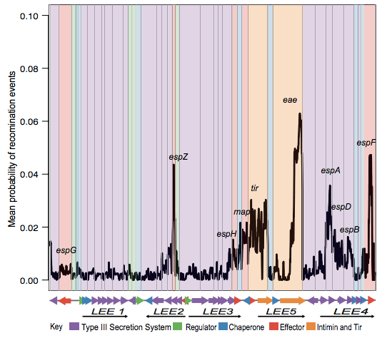
The first analysis of the genome data from this collection was reported in this 2016 paper, also in Nature Microbiology. It focused on understanding the population structure of the pathotype, including establishing a framework for looking at variation in the primary virulence locus (the LEE pathogenicity island; see blog post here).

aEPEC_distribution

Danielle then looked at serotype diversity in the collection, and used the experience to tackle the problem of O and H serotype prediction from genome data. That work is detailed in this Microbial Genomics paper, which utilises the phenotypes and genome data from the GEMS aEPEC collection to assess the reliability of predictions.

Finally we turned our attention to antimicrobial resistance (AMR) in the isolate collection – characterising resistance phenotypes, looking at known genetic determinants of AMR in the genome data, and also examining data on prescribing of antimicrobials for treatment of diarrhoeal disease in children at each study site.

So what did we find?

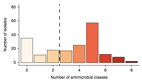
Firstly, whether we consider AMR phenotypes or genotypes we see that AMR was rampant, with most strains either multidrug resistant (65%; resistan to ≥ 3 drug classes) or susceptible to all drugs tested (19%):

AMR_classes

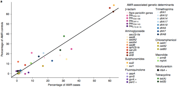
We found >40 different acquired AMR genes in the genomes, and also point mutations that are known to be associated with resistance to fluoroquinolones (in gyrA, parC) or nitrofurantoin (nfsA). Notably there was no difference between AMR rates in cases and controls, even at the level of individual genes:

genewise case control

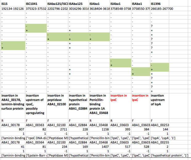
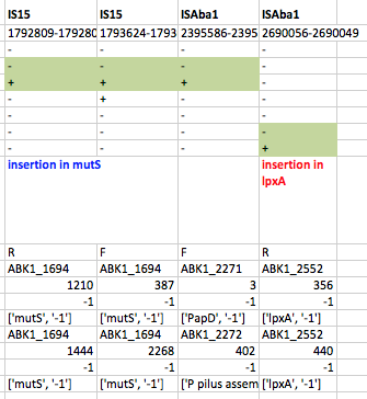
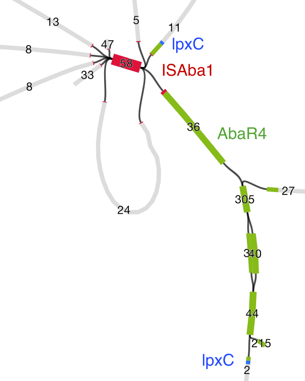
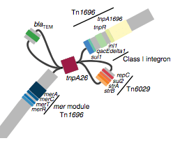
We found that many of these AMR genes co-occured together in known mobile genetic elements:

Screen Shot 2018-08-21 at 12.59.41 pm.png

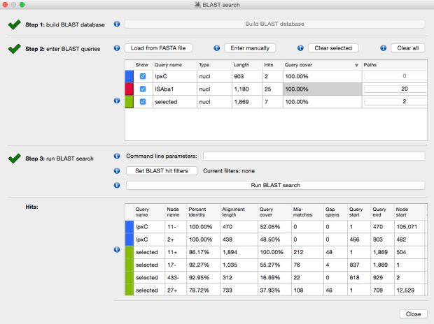
Quite often the structures of these elements were not totally resolvable from the genome assemblies, which were based on short Illumina reads only (no long reads for this data set unfortunately!)… but nevertheless, Danielle could often resolve co-localisation of these genes from the assembly graphs using Bandage:

Screen Shot 2018-08-21 at 1.00.28 pm

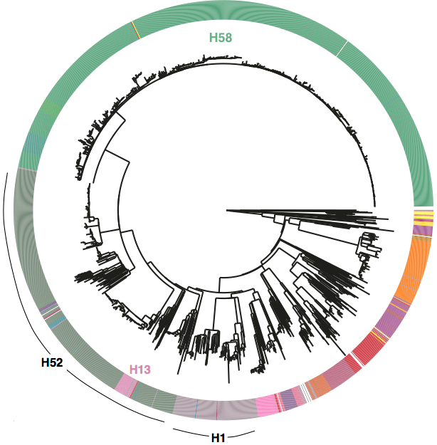
We had seen in the first paper that the isolates were highly diverse, comprising dozens of distinct clones… this tree is inferred from a core gene alignment of the study isolates together with some other genomes for context (GEMS study isolates are indicated as dark blue in the outer ring). The ten shaded clades indicate dominant clonal groups in the study population.

aEPEC_tree

Back to the AMR study. We did a discriminant analysis of principle components (DAPC) to see whether the variation in the distribution of genetic determinants amongst the genomes could be used to discriminate between the clonal groups, and saw that AMR was not associated with individual clones:

clone DAPC

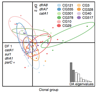
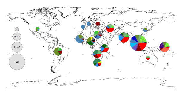
Instead we found that variation in AMR gene complement could discriminate isolates from different geographical region, suggesting that AMR genes more often reflect horizontal acquisition from distinct local gene pools in different parts of the world, rather than fixed features of their host bacterium that travel the world with their host strain (clone):

region DAPC

In particular, we saw that fluoroquinolone resistance associated mutations in gyrA were associated with Asian sites; while sites in East vs West Africa could be discriminated by the presence of different dihydrofolate reductase (dfr) genes responsible for trimethoprim resistance, with dfrA8 being more common in West Africa and dfrA5 being present in East Africa.

region gene prevalence

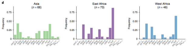
The data we have showed regional differences in AMR phenotypes, and in antibiotic usage for treatment of paediatric diarrhoea at the GEMS sites.

a) Resistance phenotypes. b) Frequency of antimicrobials prescribed to children with watery diarrhoea. c) Frequency of antimicrobials prescribed to children with dysentery.

However the prevalence of acquired resistance genes amongst E. coli isolated from each site was not associated with local frequencies of drug usage. The exception was fluoroquinolones: point mutations in gyrA and parC (which reduce MIC to ciprofloxacin) were more common at the Asian sites, where ciprofloxacin was used much more often to treat diarrheal disease than in African sites.

cipR gyrA parC

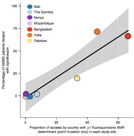
There are many possible reasons for the lack of association between local prescribing for diarrheal disease and the presence of AMR genes in local diarrheal pathogens. We expect that most antimicrobial exposure in human gut bugs like E. coli probably is not associated with attempts to treat E. coli infection at all, but with exposure to drugs given to treat other infections, drugs used in food animals which are a reservoir for E. coli, or even environmental contamination with antibiotics. Also because the horizontally acquired genes tend to travel together as a group in mobile genetic elements, exposure to one drug can co-select for resistance to many. This may be one reason that the association was more evident for ciprofloxacin use and gyrA/parC mutations, which are not in linkage with acquired AMR genes.

Finally, the data provided an opportunity to explore how well we can predict AMR phenotypes based on identifying known genetic determinants of AMR in E. coli genomes. The results were pretty good, indicating low rates of “very major errors” (where we predict a strain to be susceptible, but really it is resistant) for most drug classes. These results are comparable to those done independently in other collections of E. coli and also other bacteria, summarised here. But clearly there is room for improvement, and probably a few new mechanisms floating around out there… notably we didn’t aim to assess changes in expression of intrinsic E. coli genes, such as efflux pumps and beta-lactamases, which can contribute to drug resistance but are not so easy to find in genome data.

geno_pheno

Global genomic framework for typhoid

It’s been over a year since we published the first global whole-genome snapshot of nearly 2000 genomes of the typhoid bacterium, Salmonella Typhi in Nature Genetics.

That paper focused on the emergence and global dissemination of what we’ve been calling for years the “H58” clone (see this blog post). This clone accounted for nearly half of all the isolates sequenced, and is a big deal because it tends to be multidrug resistant (MDR), carrying a suite of resistance genes that render all the cheap, first-line drugs like chloramphenicol, ampicillin, and trimethoprim-sufamethoxazole useless for treatment. Detailed genomic epi studies show the local impact of the arrival of MDR H58 in countries as widespread as Malawi and Cambodia; and the emergence of fluoroquinolone resistant H58 sublineage in India and Nepal recently stopped a treatment trial because the current standard of care – ciprofloxacin – was resulting in frequent treatment failure.

While H58 is important, the global Typhi population contains a lot of genomic diversity outside the H58 clone, and we’ve turned our attention to the rest of the population now in a new paper in Nature Communications: “An extended genotyping framework for Salmonella enterica serovar Typhi, the cause of human typhoid”

First, we decided that we needed to revisit the haplotyping scheme of Roumagnac et al (from which H58 gets its name), which was based on just ~80 genes, using the whole genome phylogeny. Here is the tree inferred from core genome SNPs in 1832 Typhi strains, with the old haplotypes indicated by the coloured ring around the outside. It’s pretty easy to see that some haplotypes (like H52 and H1) actually comprise multiple distinct phylogenetic lineages (low resolution), while others subdivide lineages (excessive resolution).

Whole genome SNP tree for 1832 strains, outer ring indicates haplotypes based on mutations in 80 genes as defined in Roumagnac et al, Science 2006.

We used BAPS to define genetic clusters at various levels (thanks to Tom Connor for running this). We settled on 3 levels of hierarchical clustering, indicated in the tree below:

• 4 nested primary clusters (inner-most ring; yellow, green, blue, red). These have 100% bootstrap support and are each characterised by >20 SNPs

• Clusters are further divided into 16 clades (middle ring and labels). The median pairwise distance between isolates in the same clade is 109 SNPs, while the inter-clade SNP distance averages 243 SNPs.

• Clades are further divided into 49 subclades, indicated by alternating background shading colours. The median pairwise distance between isolates in the same subclade is 25 SNPs.

Fig1_noH58_clade_colours_subcladebg_190515_labelled_ED.png

Tree indicating new phylo-informed genotypes. Primary clusters 1-4 are indicated in the inner ring. Branch colours indicate clades, which are also labelled on the outside and coloured in the outer ring. Subclades are indicated by alternating background shading.

subcladerect One of the key reasons we wanted to define the phylogenetic lineages in this way is to make them easier to identify and talk about. I’ve always been a fan of MLST for this reason, since it’s much easier to talk about K. pneumoniae ST258, ST11, ST15 etc than ‘that lineage that has reference strain X in it’. So we introduce a hierarchical nomenclature system, similar to the one currently in use for Mycobacterium tuberculosis, where the 4 primary clusters (1, 2, 3, 4) are subdivided into 16 clades (1.1, 1.2; 2.1, 2.2, etc) which in turn are subdivided into 49 subclades (1.1.1, 1.1.2, etc). This has the advantage of conveying hierarchical relationships between groups – e.g. 2.2.1 and 2.2.2 are sister subclades within clade 2.2, which is a sister clade of 2.1.

The subclades are easier to distinguish in the collapsed rectangular tree on the right, where each subclade is represented by just one strain.

Some BAPS clusters were polyphyletic and consisted of isolates belonging to rare phylogenetic lineages whose common ancestor in the tree coincided with the common ancestor of an entire clade (n=9) or primary cluster (n=2). These groups contain isolates that, given increased numbers, may emerge as distinct clusters that form sister taxa within the parent clade (or primary cluster), and were given the suffix ‘.0’ rather than a defined cluster number (e.g. 3.0 or 3.1.0) to indicate non-equivalence with the properly differentiated sister clades (n=16) or subclades (n=49). As more genomes are added, these are expected to be more clearly differented into distinct groups and given proper clade/subclade designations.

Next we defined a set of 68 SNPs that can be used to genotype isolates into these groups. We chose one SNP for each primary cluster, clade and subclade (preferentially choosing intragenic SNPs in well-conserved core genes). The SNPs are detailed in a supplementary spreadsheet, and we provide a script to assign strains to genotypes based on an input BAM or VCF file generated by mapping to the reference genome for Typhi strain CT18.

An isolate that belongs to a differentiated subclade such as 2.1.4 will be hierarchically identified by carrying the derived allele for primary cluster 2 (but not the nested clusters 3 and 4); the derived allele for clade 2.1 (but no other clades) and the derived allele for subclade 2.1.4 (but no other subclades). It is possible for an isolate to carry derived alleles for a primary cluster and clade with no further differentiation into subclade.

The clone formally known as H58
Under the new scheme, the infamous H58 clone is named subclade 4.3.1, which so far has no sister clades. I suspect those of us familiar with Typhi population genomics will keep referring to it informally as H58 for some time, since that name is now well known… but I will try to re-train myself to call it 4.3.1 (H58).

Now the fun part: exploring the geographical distribution of these lineages.

Figure 1c from the paper. Pie colours indicate clades found in each WHO region in the global data set (key is in the tree figure above).

In the paper we go on to show that:
• clades are widely geographically distributed, while subclades are geographically constrained (see heatmap below);
• genotyping can be used to predict the geographical origin of travel-associated typhoid in patients in London;
• even better predictions can be obtained based on genome-wide SNP distances to our reference panel of >1800 isolates… but of course that involves a lot more computationally intensive comparisons than a quick screen of a new isolate’s BAM file.

Screen Shot 2016-08-29 at 11.47.15 pm.png

Figure 2 of the paper, showing the geographical distribution of subclades, which shows most subclades are restricted to a single region. For this analysis, the effect of local outbreaks has been minimised by replacing groups of strains that share the same subclade and year and country of isolation with a single representative strain.

You can read the full details in the paper, but here I just want to highlight that you can now explore the global genomic framework for Typhi – including genotype designations as well as temporal and geographic data – interactively in MicroReact.

Screen Shot 2016-08-29 at 11.32.21 pm.png

Geographic distribution of subclades, visualized using MicroReact. Colours correspond to the clades shown in trees above and below.

How does genotyping help with studying local populations?

We have already begun using the new genotyping scheme in local typhoid studies. I find this a really helpful way to describe/summarise the local populations, and place them in the context of the global population without resorting to large trees.

For example in this recent Nigerian study, we described the population like this: “The majority of isolates (84/128, 66%) belonged to genotype 3.1.1 , which is relatively common across Africa, predominantly western and central countries. In the wider African collection genotype 3.1.1 was represented by isolates from neighbouring Cameroon and across West Africa (Benin, Togo, Ivory Coast, Burkina Faso, Mali, Guinea and Mauritania) suggesting long-term inter-country exchange within the region. Most of the remaining isolates belonged to four other genotypes (4.1, 2.2, 2.3.1 and 0.0.3).”

Of course genotype assignment is not the end of the story – we still want to build whole-genome trees to explore the relationships of local isolates with those from other countries. Importantly, working with genotypes means that we can achieve this without needing to build a megatree of all isolates in the local + global collections (n>2000). Instead, we can use the genotypes to identify which strains from the global collection are relatives of the Nigerian isolates, and build a much smaller tree that still captures all of the information about transmission/transfer between Nigeria and other countries:

journal-pntd-0004781-g001

The tree and map were made using MicroReact, you can recreate theme here: http://microreact.org/project/styphi_nigeria To get this colour scheme just click on the eye icon (bottom left) and select ‘country’; and to get the fan style tree, click the settings button (top right) and click the fan shape.

Another example is in our recent paper on isolates collected in Thailand before and after the introduction of their national vaccination program (pre-print here):

Genotype 3.2.1 was the most common (n=14, 32%), followed by genotype 2.1.7 (n=10, 23%)
Genotypes 2.0 (n=1, 2%) and 4.1 (n=3, 7%) were observed only in 1973 (pre-vaccine period)
Genotypes 2.1.7 (n=10, 23%), 2.3.4 (n=1, 2%), 3.4.0 (n=2, 5%), 3.0.0 (n=3, 7%), 3.1.2 (n=2, 5%), were observed only after 1981 (post-vaccine period)
Genotypes 3.2.1 and 2.4.0 were observed amongst both pre- and post-vaccine isolates, but the subclade phylogenies show that these more likely to represent re-introduction of strains from neighbouring countries than persistence within Thailand throughout the immunisation program.

Genomics of atypical enteropathogenic E. coli

Well our paper on “atypical” enteropathogenic E. coli is finally out, in the new journal Nature Microbiology. The hard work on this paper was done by Danielle Ingle, whom I co-supervise together with Roy Robins-Browne and will soon become the first of my students to complete a PhD. Unfortunately the paper is paywalled at the moment, so I’ll try to summarise the key elements here.

For those who aren’t familiar with the wacky world of E. coli pathotypes, the LEE genomic island is the darling of E. coli pathogenicity genetics. It encodes a type three secretion system, essentially a syringe structure that enables the bacteria to inject its own proteins (known as secreted effector proteins) directly into human cells and – ahem – mess them up (for more technical details see the impressive body of work from Melbourne University’s very own Jacqueline Pearson and Liz Hartland). E. coli that possess shiga toxin as well as the LEE cause nasty bloody diarrhoea and are defined as enterohaemorrhagic E. coli (EHEC), while those with LEE + the bfp adhesion factor cause diarrhoea and are defined as enteropathogenic E. coli (EPEC). Strains carrying the LEE but lacking both shiga toxin and bfp can also cause diarrhoea, but are also sometimes isolated from healthy individuals with no symptoms of diarrhoaea, and it is this big group of LEE + ??? strains that are defined as atypical EPEC (aEPEC), while those with bfp are dubbed typical EPEC.

No one has been able to find a common virulence factor that differentiates diarrhoeagenic aEPEC from asymptomatic strains… which is not that surprising considering that aEPEC is really just an umbrella term for a diverse group of organisms that happen to carry the LEE genomic island.

In this paper, we set out to define the population structure of aEPEC strains using genomics, and also to investigate variation in the LEE island itself. Our strain set is ~200 newly sequenced aEPEC that were isolated from children with diarrhoea, and from asymptomatic age-matched controls, as part of the Global Enteric Multicenter Study (GEMS) – a massive study into the etiology of childhood diarrhoea across seven sites in Africa and Asia, funded by the Gates Foundation. We also included lots of publicly available genomes from NCBI, which included ~60 additional aEPEC.

So what did we find? Well from a population structure point of view, we confirmed what we suspected from the beginning – that the ~200 aEPEC strains actually represent dozens of distinct lineages or clonal groups within the E. coli whole genome phylogeny. We tried making the core genome tree in a few different ways, including mapping reads to a reference genome vs using Roary to generate core gene alignments from assemblies; with and without removing recombinant regions identified using ClonalFrameML. The alternative trees all tell the same population structure story, as you can see below. An interactive version of the mapping-based, recombination-filtered tree (which appears in Figure 1 of the paper, panel a below) is available to play with in MicroReact.

Supplementary Figure 1

The 10 clades highlighted in the tree are those containing >5 aEPEC in our collection, which represent the most common aEPEC lineages. The figures below show that these 10 aEPEC groups are present across the Asian and African GEMS sites; most also appear in non-GEMS collections from Europe as well as North and South America, indicating they are globally distributed.

aEPEC_distribution

Next we looked in depth at the LEE genomic island itself. ClonalFrame analysis identified lots of recombination across the locus, particularly affecting the proteins that make direct contact with host cells:

Screen Shot 2016-01-19 at 9.46.45 am

Danielle also did a lot of work to examine selection pressures on the various LEE genes, and found evidence for co-evolutionary constraints on groups of LEE genes (see the paper for details).

We used the recombination-free ClonalFrame tree, which represents the underlying clonal or vertical evolutionary relationships between LEE sequences, to define LEE lineages and subtypes. We also made a MLST-style scheme for the LEE, to make it easy to identify types from sequence data without having to compare to reference trees. The sequence files are included in the SRST2 distribution and can be downloaded from https://github.com/katholt/srst2.

Screen Shot 2016-01-19 at 9.50.41 am

There were three clearly distinct LEE lineages, separated from one other by 4-7% divergence (similar to genus-level differences between bacteria) and with different preferences for chromosomal insertion site. One of the LEE lineages (lineage 1) was entirely novel and we found it only in aEPEC isolates from the GEMS study. Functionality of the LEE was confirmed in all GEMS strains, including these novel lineage 1 examples.

Importantly, different aEPEC lineages had distinct LEE variants, often integrated at different chromosomal sites, confirming that aEPEC lineages have evolved numerous times independently via distinct LEE acquisition events. Also, some aEPEC lineages contained strains carrying different LEE lineages and/or subtypes, sometimes integrated at different sites, indicating ongoing evolution within some aEPEC clades.

aEPEC_tree_LEE_subtypes

Unsurprisingly, some of the “aEPEC” lineages also include examples of EHEC and/or typical EPEC isolates, i.e. subclades within the LEE-containing lineage that have subsequently acquired shiga toxin (via phage) or a bfp plasmid. We also found extensive variation in the complement of known LEE-secreted effectors (which are scattered around the genome and known as non-LEE encoded effectors or nle genes), both within and between lineages.

There’s lots more work to do to unravel the genetic basis for pathogenicity in E. coli, including identifying more of the colonisation factors, regulators and effectors that are important for causing disease in humans. But I think this analysis is a great step towards clarifying the population structure of EPEC and the LEE more generally, which opens the door for much more informative diagnostics and epidemiological studies. This work should also help immensely in guiding future pathogenicity research… most research on EPEC or EHEC pathogenicity has so far focused on a handful of strains, but our genomic analysis shows there is a much wider diversity of strain backgrounds, LEE variants and effector gene content that also needs to be considered.

Microbial Genomics methods

MGen (Microbial Genomics) was created last year by the UK’s Microbiology Society, with the aim of becoming the go-to journal for microbial genomics research. As a Senior Editor, I was asked to help mark the occasion of MGen’s six month anniversary (on Jan 15, 2016), by reviewing the 24 papers published in the journal’s first six months since launch.
The full review is is available over on the MGen site, but I wanted to draw particular attention here to trends in the analysis tools used by the genomic epidemiology papers published so far in MGen, which largely reflects what’s been happening across the field generally.

tools word cloud

One third of the articles are cutting edge genomic epidemiologyin action, using genomics to investigate the evolution and transmission of a range of pathogens, from anthrax to dysentery and food poisoning.

Interestingly all of these studies used similar methodologies, reflecting the maturity of this field of research.

Common approaches include: (i) sequencing large numbers of isolates using high-throughput Illumina platforms; (ii) the identification of SNPs (single nucleotide polymorphisms) using read mapping approaches (with BWA, SMALT, SAMtools and GATK being popular tools); and (iii) uniform use of RAxML for generating maximum likelihood phylogenies.

Some also used BEAST to estimate mutation rates, divergence dates and phylogeographical patterns. Interestingly, half of these papers utilised MLST (multi-locus sequence typing) to identify clades, showing that this sub-genomic approach based on capillary sequencing of ~7 gene fragments is still considered useful by many genomic researchers. [NOTE: nice to see that most who were inferring MLST from Illumina data were using our SRST or SRST2 software.]

Almost all of the genomic epidemiology studies took steps to remove SNPs introduced via recombination, in order to capture the underlying signals of vertical inheritance that are so important for transmission studies. Popular tools were BratNextGen, Gubbins and ClonalFrameML, which were all published within the last 3 years.

…

For pan genome analysis, Velvet and SPAdes were the most popular tools for bacterial genome assembly, with Prokka and Prodigal for gene annotation, and LS-BSR and related approaches being commonly used to cluster orthologous groups of genes.

Most of this won’t be any surprise to people working in bacterial genomic epi, but I think it’s great to see that consensus is emerging on how best to do these sorts of analyses, and to at last have some reliable tools for detecting and accounting for recombination.

The area of least agreement remains SNP calling – which mainly comes down to which read mappers to use, and which SNP calling algorithms and filtering to go with? This is a complex area, as highlighted in the recent review “Best practices for evaluating single nucleotide variant calling methods for microbial genomics” in Frontiers in Genetics, which did a very thorough job of examining the issues that need to be considered, but (quite deliberately) doesn’t provide an answer to “which tool is best?”.

Although there is still no real consensus on exact methods for SNP calling, I think most of the tools people are using (ie a good, stable read mapper followed by SNP calling with an established tool like SAMtools or GATK, with some basic filtering to remove low-evidence or ambiguous calls) end up with very similar answers (as we saw with the NGS outbreak analysis challenge session held at the ASM NGS meeting in September 2015). All in all it seems to me that the use of genomics for public health & diagnostic microbiology is in far better shape in this respect than clinical human genomics, which is going through something of a crisis involving wide discrepancies in variant calling as well as uncertainty around data interpretation.

Tracking down insertion sequences causing polymixin resistance in Acinetobacter baumannii

The first plasmid-borne colistin resistance gene was reported late last year. This was big news, but the vast majority of clinically relevant resistance to colistin and related polymixin drugs, which arises frequently in human patients being treated with these drugs, is due to de novo mutations in chromosomal genes. This has been studied quite a lot recently in Acinetobacter baumannii and Klebsiella pneumoniae, where colistin is frequently used to treat patients who are infected with carbapanem resistant strains that are also resistant to pretty much all the other antibiotics as well.

There have been quite a few studies looking for the causative mutations that underly colistin resistance in Acinetobacter and Klebsiella, by comparing the genomes of resistant and susceptible forms of the ‘same strain’ sequenced with high throughput, short read sequencing platforms like Illumina. The typical approach is to catalogue all the differences between strains and look for SNPs and other differences between them. However colistin resistance is usually associated with upregulating pmr activity via point mutations or inactivating the regulator mgrB, or by inactivating the lpx cluster in Acinetobacter. A very common way for gene inactivation to occur is by an insertion sequence (IS) hopping into the open reading frame and disrupting it. IS insertions can also cause resistance by upregulating the expression of intrinsic efflux pump or beta-lactamase genes, for example the ampC gene in A. baumannii. These insertions can be tricky to find using short read data, and are sometimes missed by regular mapping or assembly based approaches.

Luckily we now have two great tools for tracking down such mutations – ISMapper and Bandage – which were critical to tracking down polymixin resistance mutations in a recent study of A. baumannii with colleagues in Singapore. The paper is published in Antimicrobial Agents and Chemotherapy, but unfortunately is paywalled… so quick summary: basically, our clinical researcher friends in Singapore (hello Li Yang!) had 10 pairs of A. baumannii isolates, consisting of a susceptible parent isolate and a derived polymixin isolate (2 that evolved in vivo during treatment with polymixins, and 8 that evolved in vitro during polymixin exposure).

Simply screening for point mutations and deletions identified causative mutations in pmr and/or lpx clusters for 8/10 genomes, but two remained unexplained. A quick screen of the genome assemblies for IS using ISfinder identified several different IS that were present in the 10 A. baumannii genomes. However as these tend to be multi-copy in the genome, they were mostly separated into their own contigs in the assemblies. Enter ISMapper and Bandage, two open source software packages from Jane Hawkey and Ryan Wick in my lab.

First we used ISMapper to identify the locations of all IS sequences in each genome… this involves passing ISMapper each of the different IS sequences, a reference genome to compare to, and the Illumina read sets for the various strains. The isolates were all from global clones 1 or 2 (GC1, GC2), so to get the best results we used a GC1 reference genome for typing IS in the GC1 strains, and a GC2 reference for the GC2 strains. A quick tabulation of the results reveals all the locations of the various IS in each sequence. This identified differential IS insertions in lpx genes (lpxA, lpxC) in three strain pairs, including one in which no other causative mutations had been identified. There was also an IS15 insertion in the mutS gene in one isolate that had many more SNPs and deletions than the others.

ISMapper results for GC2 strain pairs, showing IS that differed within susceptible-resistant pairs.

ISMapper results for GC1 strain pairs, showing IS that differed within susceptible-resistant pairs.

Cool! But what about that one last pair, where ISMapper didn’t find any differences at all between the resistant and susceptible read sets? This time we turned to Bandage, to inspect the genome assemblies and see if we could find a smoking gun. Now we had a clear hypothesis too – we were looking explicitly for interruptions in lpx genes. So we created new assemblies for these read sets using SPAdes. We loaded the graph of the susceptible isolate in Bandage first, and used the inbuilt BLAST search to locate the lpx genes within the graph – all were intact as expected, sitting happily in the middle of long contigs.

Contig containing the lpxC gene (blue) in SPAdes assembly of the susceptible isolate

Then we loaded the graph of the polymixin resistant isolate in Bandage first, and did the BLAST searches. The pmrB locus was intact, but the lpxC gene was interrupted. Very interrupted! No wonder ISMapper didn’t find this as it’s not an IS insertion at all, but rather the gene is interrupted by a large sequence, in an event that appears to involved the translocation of the entire genomic resistance island AbaR4 into the middle of the lpxC open reading frame.

Interruption of lpxC associated with movement of the antibiotic resistance related genomic island, AbaR

The above image is created by doing BLAST searches (within Bandage) for the lpxC gene, AbaR4 gene and ISAba1 gene like this…

BLAST search within an assembly graph using Bandage

…and then selecting ‘BLAST hits (solid)’ under the ‘Graph display’ settings on the left hand side of the Bandage viewer.

Screen Shot 2016-01-12 at 6.58.17 pm

Oh and just in case you think this is a weird one-off event that maybe you don’t need to worry about in your own genome data… check out the recent report from Scott Beaston and David Paterson in Queensland, who sequenced a nasty Klebsiella strain that was resistant to everything under the sun including carbapenems and colistin. They sequenced the genome with PacBio, and found the ISEcp1–bla_OXA-181 mobile element (which confers resistance to carbapenems) inserted into the mgrB regulatory gene in the chromosome, whose inactivation is responsible for colistin resistance. Oh and they also found another mobile element, ISEcp1–bla_CTX-M-15, inserted into the gene ompK35. Guess what inactivating this gene gives you? Cephalosporin resistance.