software

Bandage – View and navigate assembly graphs

New from Ryan Wick, a wonderful MSc (Bioinformatics) student in the lab:

Bandage – Bioinformatics Application for Navigating De novo Assembly Graphs Easily

http://rrwick.github.io/Bandage/

De novo assembly graphs contain assembled contigs (nodes) but also the connections between those contigs (edges), which are not easily accessible to users. Bandage is a program for visualising assembly graphs using graph layout algorithms. By displaying connections between contigs, Bandage opens up new possibilities for analysing de novo assemblies that are not possible by looking at contigs alone.

BLAST searches of an assembly can be conducted within Bandage… the resulting hits are highlighted in the graph!

Note: works with the assembly graphs output by Velvet, SPAdes and Trinity.

Tools for bacterial comparative genomics

Yesterday I spoke at a workshop for JAMS TOAST (Sydney’s Joint Academic Microbiology Seminars – bioinformatics workshop)… I was asked to cover tools for comparative genomics, so I put together a list of the tried and tested programs that I find most useful for this kind of analysis. So here is the list.

First, a few caveats…

These are mostly tools with a graphical user interface (mostly Java based)… this means they should be pretty accessible to most users, however if you want to do analyses that are a bit more custom or niche, you will have to get your hands dirty and use the commandline (which you should learn to do anyway!!)

These tools are useful for small-ish scale genomic comparisons, in the order of 2-20 genomes.

Most of these tools are for assembled data, hence we start with how to assemble your data… this will become less of an issue as we move to long read sequencing with PacBio and MinION etc, but for the moment most of the data I work with is from large scale sequencing projects with Illumina (100s-1000s) so we use mapping-based approaches for a lot of tasks… so I have included a few comments about this at the end.

Beginner’s guide with walk-through tutorial

Some of these tools, particularly the visualisation of whole genome comparisons (using Artemis & ACT, Mauve, and BRIG) are covered the in the tutorial from our 2013 “Beginner’s guide to comparative bacterial genome analysis using next-generation sequence data“. So if you want a walk-through, that’s a good place to start. Note that we have updated the tutorial (as of July 2017) to version 2, available here.

First things first – Are my reads good quality?

FastQC – Generate graphical reports of read quality from the fastq files.

Assembly

SPAdes – de Bruijn graph assembly, incorporating multiple kmers and read pairing information in the building of the graph. Think of this as a more sophisticated version of Velvet… in my experience, it nearly always provides better assemblies than Velvet, except on the rare occasion (1-5% of read sets) where it fails to get a good assembly at all. In which case, try Velvet!

Velvet – The first and most widely used de Bruijn graph assembler built to tackle the problem of short reads. Graphs are built using a single kmer value, and read pairing information used for scaffolding only (unlike SPAdes, where multiple kmers are incorporated into a single graph and read pairing is also used directly in building the graph). How do you know what kmer to use? Use Velvet Optimiser. Hate the command line? Try Vague, a GUI wrapper for Velvet.

How do I judge if I have a good assembly? Try QUAST

What other assemblers are there? What’s best for what task? Take a look at Nucelotid.es and Assemblathon.

How can I view my assembly graphs? Try Bandage – freshly released from Ryan Wick, a MSc (Bioinformatics) student in my lab. Bandage allows you to view and manipulate de Druijn graphs output by Velvet or SPAdes… lots of super cool features and useful applications, see the github site for examples.

Working with assembled data

Now you have a nice set of assembled contigs – where are all the genes?

Whole genome annotation

RAST – Web tool (upload contigs), uses the subsystems in the SEED database and provides detailed annotation and pathway analysis. Takes several hours per genome but I think this is the best way to get a high quality annotation (if you have only a few genomes to annotate).

Prokka – Standalone command line tool, takes just a few minutes per genome. This is the best way to get good quality annotation in a flash, which is particularly useful if you have loads of genomes or need to annotate a pangenome or metagenome. Note however that the quality of functional information is not as good as RAST, and you will need several extra steps if you want to do functional profiling and pathway analysis of your genome(s)… which is in-built in RAST.

Annotating specific types of features

Resistance genes

CARD – best combination of easy interface + pretty good database
ARG-Annot – best quality database (in my experience, focusing on Enterobacteriaceae)
ResFinder – easy interface, database needs ongoing development

Virulence genes

PATRIC – for certain bugs only, but has good online tools for genome comparisons.
VFDB – broader range of species, but varying levels of comprehensiveness and you need to do more of the work yourself.

Insertion sequences

IS saga – Upload your genome and have IS saga find all the transposes in your genome using their IS finder database

Phage

PHAST – Upload your genome and this will identify likely prophage regions, summarising these at the level of whole phage and also individual genes.

Viewing your genome – The Artemis Genome Browser

There are zillions of genome browsers out there, but I still love Artemis… and not just because I’m from the Sanger Institute. Unlike most genome browsers, Artemis was custom-built for bacterial genomes, which let’s face it are really quite different from humans and other eukaryotes.

The default view shows you your sequence and annotation, with 6 frame translation and allows you to easily edit or create features in the annotation, graph sequence-based functions like GC content and GC skew, and do all manner of other useful things. It’s been around for a zillion years (well, at least 10 or so) and is very well developed and supported.

Artemis has lots of cool features built in, including the ‘BamView’ feature that allows you to view BAM files that show the alignment of reads mapped to your genome, zoomed in to the base level or zoomed out to look at coverage and SNP distributions… this is also super handy for viewing RNAseq data, as you can easily see the stacks of reads derived from coding regions.

Artemis also has DNA Plotter built in, which you can use to generate those pretty circular figures of your genome sequences and their features.

Plus, when you’ve got used to using Artemis to get to know your shiny new genome, you can move on to viewing comparisons against other genomes using ACT – the Artemis Comparison Tool.

Comparing whole genome assemblies

NOTE: Walk-throughs of these tools, using examples from the 2011 E. coli outbreak in Germany, are covered in the “Beginner’s guide to comparative bacterial genome analysis using next-generation sequence data“.

ACT (Artemis Comparison Tool) – Visualises BLAST (or similar) comparisons of genomes. This is most useful for comparisons of two or a few genomes, and makes it easy to spot and zoom in to regions of difference.

Mauve – Whole genome alignment and viewer that can output SNPs, regions of difference, homologous blocks, etc. It can also be used to assess assembly quality against a reference, using Mauve Contig Metrics.

BRIG (BLAST Ring Image Generator) – Gives a global view of whole genome comparisons by visualising BLAST comparisons via pretty circular figures. This is suitable for comparing lots of genomes, although because you have to enter each one through the GUI, it’s tricky to do more than a dozen or so.

Whole genome SNP-based phylogenies (from assembled data)

You can’t go past Adam Phiippy’s Harvest Suite

Parsnp – Compare genomes to a reference (using MUMmer) to identify core genome SNPs and build a phylogeny

Gingr – View the phylogeny and associated SNP calls (VCF format)… also useful for visualising tree + VCF that you have created in other ways, e.g. from mapping.

Detecting recombination in whole genome comparisons

Gubbins – A new implementation of the approach first used in Nick Croucher’s 2011 Science paper on Streptococcus pneumoniae. Command-line driven and runs pretty fast (<2 hours usually on our data).

BRAT NextGen – Uses a similar idea to Gubbins but using Bayesian clustering is GUI-driven… sounds nice, but actually I find it less convenient than Gubbins as there are manual steps required and then you need to run lots of iterations to get significance values.

Mapping based analyses

Why?

If you have specific questions to answer, where precise variant detection is important (e.g. allele calling, MLST, SNP detection, typing, mutation detection), mapping provides greater sensitivity and specificity than assembled data. Basically, if you want to be really sure about a variant call, you should be using the full information available in the reads rather than relying on the assembler and consensus base caller to get things right every time. See our SRST2 paper if you don’t believe me.

Also, if you need quick answers to specific questions, this is almost always going to be achieved faster and more accurately if you work direct from reads without attempting to generate high quality assemblies first.

The basics

For mapping our go-to is BWA or Bowtie2 (getting from fastq -> BAM). For processing of BAMs we use: SAMtools and BAMtools for variant calling, and BAMstats and BEDtools for summarising coverage and other information from the alignments.

Pipelines for specific tasks

There are loads of pipelines around the place that use the basic tools above to do specific tasks. A few of ours are:

SRST2 – MLST, resistance genes, virulence genes
ISMapper – IS (insertion sequence / tranposase) insertions
RedDog – Whole genome SNP-based phylogenies

Behind the paper: SRST2 for short read sequence typing of bacterial pathogens

[Originally posted by Kat on her BacPathGenomics blog, Nov 2014]

I’m pleased to say our paper SRST2: Rapid genomic surveillance for public health and hospital microbiology labs is now out in the Genome Medicine/Genome Biology special issue Genomics of Infectious Diseases!

Having posted the code to GitHub over a year ago, and the paper to BioRxiv in June, it is great to have it finally published. I must say I love the BioRxiv experience, it is great to know the paper was viewed >1500 times while it was stuck in the peer review/publication process.

This project has been a fun journey, which started when I was lucky enough to get a fantastic summer intern, Harriet Dashnow (follow: @hdashnow), funded by VSLCI (our wonderful local supercompute cluster). Harriet’s job was to figure out how to apply our SRST code, which was designed to extract MLST information from Illumina reads (see code and BMC Genomics paper), to detect and type resistance genes and alleles. She did a fantastic job, but in doing so we realised that we needed to overhaul the scoring system to something that was faster and more robust. So, Mike Inouye designed a new scoring approach from the ground up, which Harriet and Bernie Pope from VLSCI turned into the new Python code that is SRST2. We then did a whole lot of testing on public data (mainly by Lesley Raven and Mark Schultz from the Holt & Inouye labs, with some guidance from Justin Zobel in the Computing & Info Systems department) and had our friends at the local reference lab, the Microbiological Diagnostic Unit (mainly Takehiro Tomita), test it out for themselves on a load of Listeria monocytogenes they had recently sequenced on their MiSeq.

What we came up with was some code that draws on the fundamental tools of the genomics trade (bowtie2, samtools & python) to rapidly and reliably detect genes and alleles direct from short read data. SRST2 has two modes, (i) MLST, where you can provide MLST alleles and profile definitions, and it will report sequence types; and (ii) gene detection and allele calling, suitable for screening for acquired genes such as resistance genes, virulence genes and/or plasmid genes.

Figure 1 from the paper outlines how SRST2 works:

The coolest thing about SRST2 is that it is consistent and reliable, even at low read depths, which is absolutely critical for use in a routine diagnostic/surveillance workflow. The robustness of SRST2 stems from the fact that we use a mapping approach coupled with a pretty clever approach to scoring potential matches.

The alternative is to generate de novo assemblies, and then interrogate them with BLAST or other tools… the problem with that approach is that, while de novo assemblers like Velvet and SPAdes can do a great a job of assembling bacterial genomes, there is no way to guarantee you will get a good assembly with every read set. Anyone who works with biggish bacterial data sets of 100s-1000s of genomes knows – it is very hard to standardize the assembly process and establish a protocol that works consistently and reliably every time. And if you are needing to type loads of strains as part of routine service or investigations, you need to know you will get a reliable result every time. Figure 3 in the paper compares the overall performance (call rate x accuracy) of SRST2 vs BLAST analysis of highly optimised assemblies:

As you can see, once you get up to 15-20x read depth, SRST2 will consistently give you an answer, and that answer will be accurate. Whereas using assemblies – even highly optimised ones – you will always miss out on 1-5% of the answers.

We were also asked by a reviewer to compare SRST2 with the only other publicly-available program designed for MLST typing from short reads: the MLST Typer web service at the Danish Center for Genomic Epidemiology. Because this requires uploading read sets to the other side of the world, we only did this for one of our test data sets, 44 Salmonella genomes. The results are in Table 5, and showed that the website got the correct ST for only 14/44 genomes. SRST2 got correct STs for 43/44 genomes (for the 44th strain, SRST2 returned 6/7 alleles correctly and suggested that there is actually a SNP in the 7th allele, which could actually be correct but we cannot verify; MLST Typer did not call anything for this strain).

When it comes to detecting the presence of genes, such as acquired antibiotic resistance genes, SRST2 also outperformed assembly based approaches. We got accurate detection at depths >3x, and picked up many resistance genes that did not assemble well, especially at depths below 15x (see Fig 5 of the paper). Again, we compared to ResFinder on the Center for Genomic Epidemiology website, and found SRST2 performs much better (see Table 3 in the paper). I don’t want to criticize the tools on the Center for Genomic Epidemiology website, as they are really useful for people who have limited resources to analyse genome data… but I do think people need to be aware that the successful use of those tools rely heavily on first obtaining a high quality assembly, and you can very easily miss important antibiotic resistance genes.

So what are the main uses for SRST2?

The key jobs SRST2 is good for are:

detecting the presence of genes
identifying specific alleles for those genes from a known set of sequencescalculating sequence types (STs) specified by MLST-style schemas.

So it is great for detecting acquired genes, such as antibiotic resistance genes, virulence genes or plasmid genes; or extracting MLST information. To this end, the SRST2 download includes:

a script to help you pull down the latest MLST data from pubmlst.org for >100 MLST schemes
instructions and code for typing virulence genes from the Virulence Factor Database (VFDB)
SRST2-compatible versions of popular resistance gene databases (ARG-Annot, ResFinder) and the PlasmidFinder database of plasmid replicons

For example, in the paper we show the use of SRST2 for investigating changing patterns of vancomycin resistance amongst Enterococcus faecium isolated at a local hospital (data from this 2013 MBio paper). We analysed the Illumina readsets using SRST2 to detect resistance genes and perform MLST. SRST2 returned a table of strains with columns to indicate sequence types, alleles for each locus in the MLST scheme, and the presence of acquired resistance genes (shown here viewed in Excel):

You will notice that the depth values are VERY high for this data set, as the sequencing was done at relatively low-plex on a HiSeq. This means that it takes a long time to map (and VERY long time to assemble) these read sets… however note that you can obtain the same results much faster by telling SRST2 to use just the first 1 or 2 million reads per strain, which is more than enough to get accurate results (–stop_after 1000000).

We used R to summarize and plot the results, which are shown in Figure 7 in the paper (R code is in the /scripts directory in the SRST2 download):

Panel (a) shows that vanB vancomycin resistance became more frequent over the 12 years investigated, while panel (b) shows that the STs also changed during this time period… so is the increase in resistance linked to the introduction of new van-resistant ST252 and ST203 strains?

Panel (c) puts the ST & resistance results together… the tree on the left is a dendrogram depicting the similarity between sequence types based on number of shared alleles; MLST profiles (STs and their component alleles) are shown next to this. On the right, the frequency of each ST is shown as a bar graph, which highlights that there are 3 main types, ST17, ST252 and ST203, which all share 5-6 alleles. The heatmap in the middle shows the frequency of the various resistance genes within each ST – it is clear that the vanB locus is present in all 3 STS, but only at ~50% in each… so the increase in vancomycin resistance is not explained by the introduction of resistant ST252 and ST203 clones; rather, vancomycin resistance comes and goes, via movement of the vanB operon, in all 3 common STs.

The whole genome phylogenetic analysis in the 2013 MBio paper shows this in much finer detail of course; but the basic conclusions could be drawn from a very rapid analysis with SRST2.

The same is true for hospital outbreak investigations (see examples in the paper) – in a few minutes SRST2 can show whether a potential transmission case has the same ST and acquired genes profile as confirmed outbreak cases; if the ST matches, genome-wide SNP trees can be used to investigate further.

My next post will have some pro tips for using SRST2.

Bacterial genomics tutorial

UPDATE: Version 2 of the tutorial (posted July 2017) is available here.

[Originally posted by Kat on her BacPathGenomics blog, April 2013]

This is a shameless plug for an article and accompanying tutorial I’ve just published together with David Edwards, my excellent MSc Bioinformatics student from the University of Melbourne. The accompanying tutorial is available here.

The idea for this came from discussions at last year’s ASM (Australian Society of Microbiology) meeting, where it was highlighted that there was a lack of courses and tutorials available for biologists to learn the basics of genomic analysis so that they can make use of next gen sequencing. Michael Wise, a founding editor of BMC Microbial Informatics and Experimentation based at UWA in Perth, suggested the new journal would be an ideal home for such a tutorial… so here we are:

Beginner’s guide to comparative bacterial genome analysis using next-generation sequence data

http://www.microbialinformaticsj.com/content/3/1/2/

High throughput sequencing is now fast and cheap enough to be considered part of the toolbox for investigating bacteria, and there are thousands of bacterial genome sequences available for comparison in the public domain. Bacterial genome analysis is increasingly being performed by diverse groups in research, clinical and public health labs alike, who are interested in a wide array of topics related to bacterial genetics and evolution. Examples include outbreak analysis and the study of pathogenicity and antimicrobial resistance. In this beginner’s guide, we aim to provide an entry point for individuals with a biology background who want to perform their own bioinformatics analysis of bacterial genome data, to enable them to answer their own research questions. We assume readers will be familiar with genetics and the basic nature of sequence data, but do not assume any computer programming skills. The main topics covered are assembly, ordering of contigs, annotation, genome comparison and extracting common typing information. Each section includes worked examples using publicly available E. coli data and free software tools, all which can be performed on a desktop computer.

Four great tools

In the paper and tutorial, we introduce the four tools which we rely on most for basic analysis of bacterial genome assemblies: Velvet, ACT, Mauve and BRIG. All except ACT were developed as part of a PhD project, and have endured well beyond the original PhD to become well-known bioinformatics tools. New students take note!

In the paper, each tool is highlighted in its own figure, which includes some basic instructions. This is reproduced below, but is covered in much more detail in the tutorial that comes with the paper (link at the bottom).

1. Velvet for genome assembly

Possibly the most popular and widely used short read assembler, developed by the amazing Dan Zerbino during his PhD at EBI in Cambridge. Quite a PhD project!

[ Download | Paper | Protocol ]

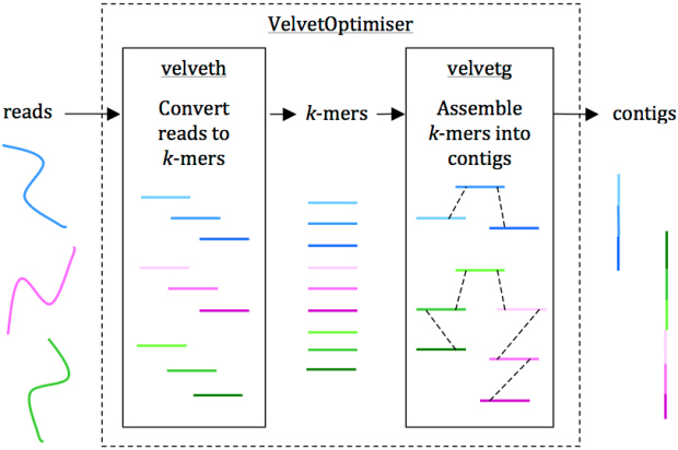
Reads are assembled into contigs using Velvet and VelvetOptimiser in two steps, (1) velveth converts reads to k-mers using a hash table, and (2) velvetg assembles overlapping k-mers into contigs via a de Bruijn graph. VelvetOptimiser can be used to automate the optimisation of parameters for velveth and velvetg and generate an optimal assembly. To generate an assembly of E. coli O104:H4 using the command-line tool Velvet:

• Download Velvet [23] (we used version 1.2.08 on Mac OS X, compiled with a maximum k-mer length of 101 bp)

• Download the paired-end Illumina reads for E. coli O104:H4 strain TY-2482 (ENA accession SRR292770)

• Convert the reads to k-mers using this command:

velveth out_data_35 35 -fastq.gz -shortPaired -separate SRR292770_1.fastq.gz SRR292770_2.fastq.gz

• Then, assemble overlapping k-mers into contigs using this command:

velvetg out_data_35 -clean yes -exp_cov 21 -cov_cutoff 2.81 -min_contig_lgth 200

This will produce a set of contigs in multifasta format for further analysis. See Additional file 1: Tutorial for further details, including help with downloading reads and using VelvetOptimiser.

2. ACT for pairwise genome comparison

Part of the Sanger Institute’s Artemis suite of tools. Also look at Artemis (single genome viewer), DNA Plotter (which can draw circular diagrams of your genomes) and BAMView (which can display mapped reads overlaid on a reference genome), they are all available here.

[ Download | Paper | Manual ]

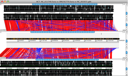
Artemis and ACT are free, interactive genome browsers (we used ACT 11.0.0 on Mac OS X).

• Open the assembled E. coli O104:H4 contigs in Artemis and write out a single, concatenated sequence using File -> Write -> All Bases -> FASTA Format.

• Generate a comparison file between the concatenated contigs and 2 alternative reference genomes using the website WebACT.

• Launch ACT and load in the reference sequences, contigs and comparison files, to get a 3-way comparison like the one shown here.

Here, the E. coli O104:H4 contigs are in the middle row, the enteroaggregative E. coli strain Ec55989 is on top and the enterohaemorrhagic E. coli strain EDL933 is below. Details of the comparison can be viewed by zooming in, to the level of genes or DNA bases.

3. Mauve for contig ordering and multiple genome comparison

Developed by the wonderful Aaron Darling during his PhD, he is now Associate Professor at University of Technology Sydney. Also see Mauve Assembly Metrics, an optional plugin for assessing assembly quality which was developed for the Assemblathon.

[ Download | Paper | User Guide ]

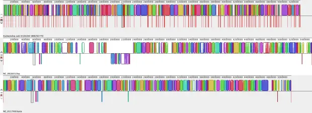
Mauve is a free alignment tool with an interactive browser for visualising results (we used Mauve 2.3.1 on Mac OS X).

• Launch Mauve and select File -> Align with progressiveMauve

• Click ‘Add Sequence…’ to add your genome assembly (e.g. annotated E. coli O104:H4 contigs) and other reference genomes for comparison.

• Specify a file for output, then click ‘Align…’

• When the alignment is finished, a visualization of the genome blocks and their homology will be displayed, as shown here. E. coli O104:H4 is on the top, red lines indicate contig boundaries within the assembly. Sequences outside coloured blocks do not have homologs in the other genomes.

4. BRIG (BLAST Ring Image Generator) for multiple genome comparison

From Nabil-Fareed Alikhan at the University of Queensland, also as part of a graduate project, which I believe is still in progress…

[ Download | Download BLAST | Paper | Tutorial ]

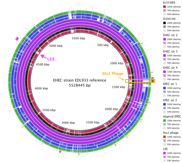
Fig4_BRIG

BRIG is a free tool that requires a local installation of BLAST (we used BRIG 0.95 on Mac OS X). The output is a static image.

• Launch BRIG and set the reference sequence (EHEC EDL933 chromosome) and the location of other E. coli sequences for comparison. If you include reference sequences for the Stx2 phage and LEE pathogenicity island, it will be easy to see where these sequences are located.

• Click ‘Next’ and specify the sequence data and colour for each ring to be displayed in comparison to the reference.

• Click ‘Next’ and specify a title for the centre of the image and an output file, then click ‘Submit’ to run BRIG.

• BRIG will create an output file containing a circular image like the one shown here. It is easy to see that the Stx2 phage is present in the EHEC chromosomes (purple) and the outbreak genome (black), but not the EAEC or EPEC chromosomes.

Tutorial

The tutorial accompanying the article is available here. To give you an idea of what’s covered, here is the table of contents:

1. Genome assembly and annotation…………………………………………………………… 2

1.1 Downloading E. coli sequences for assembly…………………………………………….. 2

1.2 Examining quality of reads (FastQC)………………………………………………………… 2

1.3 Velvet – assembling reads into contigs………………………………………………………. 4

1.3.1 Using VelvetOptimiser to optimise de novo assembly with Velvet………….. 6

1.4 Ordering contigs against a reference using Mauve………………………………………. 7

1.4.1 Viewing the ordered contigs (Mauve)………………………………………………… 10

1.4.2 Viewing the ordered contigs (ACT)……………………………………………………. 13

1.5 Mauve Assembly Metrics – Statistical View of the Contigs………………………… 15

1.6 Annotation with RAST……………………………………………………………………………. 15

1.6.1 Alternatives to RAST………………………………………………………………………. 19

2. Comparative genome analysis……………………………………………………………….. 20

2.1 Downloading E. coli genome sequences for comparative analysis………………. 20

2.2 Mauve – for multiple genome alignment……………………………………………………. 21

2.3 ACT – for detailed pairwise genome comparisons……………………………………… 24

2.3.1 Generating comparison files for ACT…………………………………………………. 24

2.3.2 Viewing genome comparisons in ACT……………………………………………….. 27

2.4 BRIG – Visualizing reference-based comparisons of multiple sequences……… 29

3. Typing and specialist tools……………………………………………………………………. 34

3.1 PHAST – for identification of phage sequences…………………………………………. 34

3.2 ResFinder – for identification of resistance gene sequences………………………… 34

3.3 Multilocus sequence typing…………………………………………………………………….. 34

3.4 PATRIC – online genome comparison tool………………………………………………… 34

Holt Lab

microbial genomics