Well, after almost 6 years, our Klebsiella pneumoniae genomics paper is finally out!
It’s a beast of a thing and there are still a million and one questions to address just from this one data set. For those interested in looking at the data for themselves, the raw reads are available under accession ERP000165, the assemblies are in Sylvain Brisse’s Klebsiella pneumoniae BIGSdb at the Pasteur Institute, and the tree + metadata are available for your interactive viewing pleasure in MicroReact.
The paper itself is open access in PNAS, you can read it here.
Genomic analysis of diversity, population structure, virulence, and antimicrobial resistance in Klebsiella pneumoniae, an urgent threat to public health

Whole genome diversity in K. pneumoniae
There have been lots of really nice Klebs genomics papers out in the last 18 months or so, examining the evolution of the ST258 clone that carries the KPC gene (K. pneumoniae carbapaenemase) and is wreaking havoc in hospitals all over the place (including recently in Melbourne), and also several hospital-based studies tracking transmission and evolution of local drug-resistant outbreaks.
But that is just the tip of the K. pneumoniae iceberg.
Our paper asks a completely different set of questions, which you could basically sum up as “what the hell is Klebsiella pneumoniae anyway?”
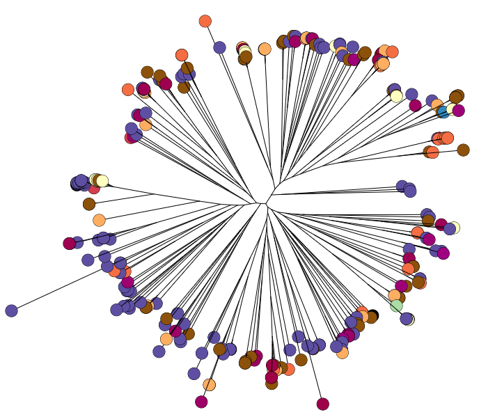
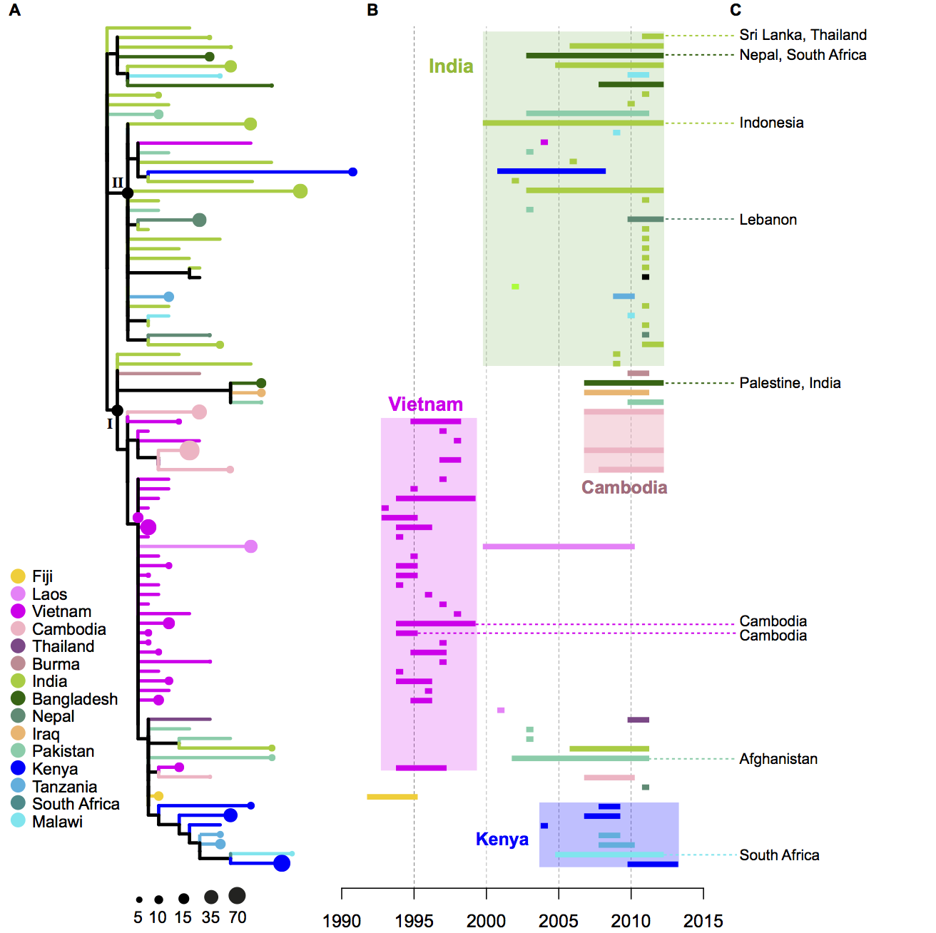
To do this, we sequenced ~300 genomes of really diverse K. pneumoniae strains. We didn’t have much information about genetic diversity to go on, so we chose strains with different phenotypes (antimicrobial resistance patterns, capsular serotypes or sequence types where known), from different sources (human and animal, asymptomatic carriage and infections of various kinds), and from different geographical locations.
This was done by an international group of collaborators who pooled their resources, not only sharing their precious strain collections but also digging through hospital and other records to find as much information about the strains as possible.
You can view the tree and associated metadata, including geographical origin and source information, over on Microreact.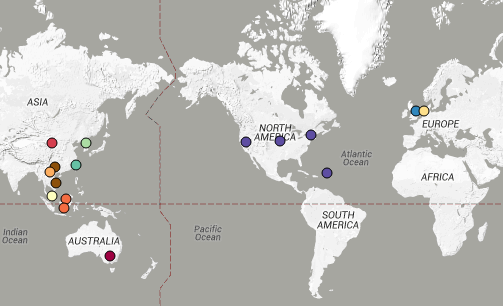
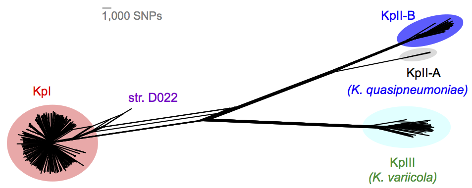
We found out some pretty interesting things about Klebsiella pneumoniae, including the fact that what’s identified as K. pneumoniae using standard tests is actually a mixed bag of three related species, that now have their own names: K. pneumoniae (KpI group, which includes the majority of clinical isolates and all the stuff you might have heard of like the clone that causes rhinoscleromatis, and the KPC clone ST258, and the hypervirulent clone ST23); K. quasipneumoniae; and K. variicola (plant associated and usually nitrogen-fixing).
By now, this species stuff has been nutted out (mainly by co-author Sylvain Brisse from Institut Pasteur) by analysing marker gene sequences, but it’s really important to be able to show that those patterns hold at the whole-genome level, and we found some interesting things about the distribution of the rarer species (see the paper for details).

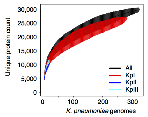
Importantly, we did the whole pan-genome analysis thing and found that as a population, K. pneumoniae has more genes than humans. Almost 30,000 in fact. Each individual strain has ~5,500 genes, but <2,000 of those are core genes that are common to all K. pneumoniae. The rest are accessory genes that can come and go, helping the bug to adapt to new environments.
One of the cool things we were able to do with our data set, which you just can’t do with genomic studies focused on specific clones or outbreaks, was to look at statistical associations between accessory genes and phenotypes. Admittedly our available phenotypes were pretty limited, but we found a few important things.
1. VIRULENCE
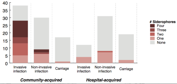
We screened for genes associated with virulence in humans by focusing in on invasive infections, and comparing gene frequencies in human isolates from invasive community-acquired infections (i.e. the kind of infections that land you in hospital) vs. those in human carriage isolates or hospital acquired infections (i.e. the kind of infections that get you when you are already in hospital for something else and are particularly vulnerable to infection).
The only genes that were significantly associated with invasive infection in humans were rmpA and rmpA2, which upregulate capsule production, and genes related to iron acquisition (specifically acquired siderophore systems that can help to steal iron from animal hosts – see paper for details). These genes have been known about for some time, based on mouse models and knowledge of other pathogens, however we were able to show that these genes are significantly associated with invasive K. pneumoniae disease in humans, which is not something that can be proven directly using experimental systems. (The siderophore story actually goes a bit deeper than the iron issue… it’s a bit too complex to go into here but I recommend reading Michael Bachman’s work e.g. “Interaction of lipocalin 2, transferrin, and siderophores determines the replicative niche of Klebsiella pneumoniae during pneumonia” in MBio, 2012).
Interestingly, doing the same test in bovine isolates showed that the story is very different: we had a lot of isolates from dairy herds, including clinical and subclinical mastitis; asymptomatic carriage isolates and strains from the farm environment… and found that an acquired lactose operon was almost perfectly associated with mastitis in cows! Something similar has been observed before in Streptococcus agalactiae.
2. ANTIBIOTIC RESISTANCE
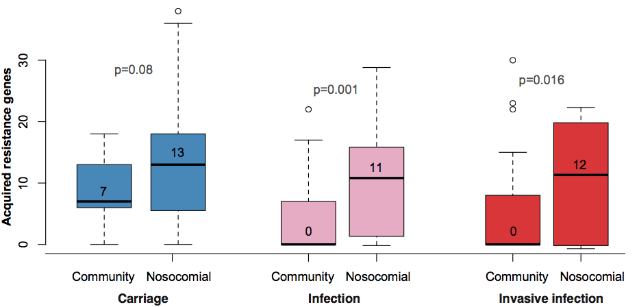
Resistance genes were associated with human hospital isolates and human carriage isolates. This is far from an ideal study design to test this, as we had different types of collections from different geographical regions; however, even when you look within different local collections you see the same patterns: (a) comparing bovine and human isolates from NY state, the resistance genes were all in human isolates not cow isolates; (b) comparing human carriage and infection isolates (both nosocomial and community acquired) in Vietnam, the resistance genes were mainly in human carriage and hospital isolates, not in community infections; (c) in the remaining countries, isolates from infections acquired in hospital had more resistance genes than those that were considered nosocomial (diagnosed within 48 hours of admission).

What’s really interesting is that while resistance genes and virulence genes are both highly mobile components of the accessory genome, they were essentially orthogonal in their distribution. The resistance genes were mainly in hospital acquired infections and carriage isolates, whereas the virulence strains were mainly found in isolates from community acquired infections.
 So far, this has resulted in the emergence of two very different kinds of K. pneumoniae clones of importance to human health: hypervirulent clones, and multidrug resistant clones. This is pretty lucky, as it means the hypervirulent clones are generally sensitive to antibiotics (although antimicrobial treatment is difficult for some conditions, like liver abscess), and the problem of untreatable highly drug resistant Klebs infections has not spread outside of hospitals.
Unfortunately, our luck appears to be runnning out and we are already starting to see the convergence of virulence and resistance. Hypervirulent ST23 strains, which have all four of the acquired siderophore systems, are accumulating antibiotic resistance genes. And about half of the KPC Klebs ST258 strains causing problems in hospitals globally have one of the siderophore gene clusters, yersiniabactin, which has been shown in clinical ST258 isolates to confer enhanced ability to cause pneumonia. How long till the other virulence genes creep in? We need to be watching!
Also, our data indicates that there are plenty of other hypervirulent or multidrug resistant Klebs clones emerging out there… convergence of virulence and resistance could happen in any one of them, so we need to be thinking and monitoring beyond the well-known ST23 and ST258 strains.
In any case, genomic surveillance is going to become really important for Klebsiella…
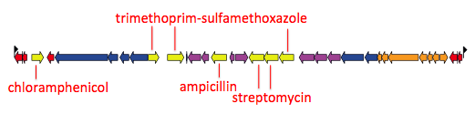


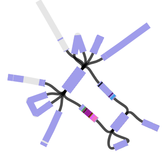
 When I use Bandage to blast for the IncHI1 plasmid sequence (hits in blue) as well as the MDR locus genes, it’s pretty easy to see that the MDR locus is located in the plasmid:
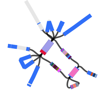


